Bank Marketing

Introduction
The data is sourced from the UCI ML Repository and can be downloaded here. It is related to the direct marketing campaigns of a Portuguese banking institution. The campaigns were based on phone calls. Multiple datasets are provided, however this analysis focuses on the full dataset (bank-addidtional-full.csv), which is also the latest and has the most number of inputs.

Goal
The classification goal is to predict if the client will subscribe (yes/no) a term deposit (variable y).

Data Dictionary

Attribute Name	Type	Description
*age*	numeric	age of the person called
*job*	categorical	type of job
*marital status*	categorical	married, single or unknown
*education*	categorical	educational attainment
*default*	categorical	has credit in default?
*housing*	categorical	has housing loan?
*loan*	categorical	has personal loan?
*contact*	categorical	contact communication type
*month*	categorical	last contact month of year
*day_of_week*	categorical	last contact day of week
*duration*	numeric	last contact duration in seconds. The duration is not known before the call, so even though this has a strong impact on outcome (duration=0 => y=0), it should be discarded from the model
*campaign*	numeric	number of contacts performed during this campaign for this client (includes last contact)
*pdays*	numeric	number of days passed since client was contacted since the client was last contacted from a previous campaign. 999 means not previously contacted
*previous*	numeric	number of contacts performed during this campaign for this client
*poutcome*	categorical	outcome of the previous marketing campaign
*emp.var.rate*	numeric	employment variation rate - quarterly indicator
*cons.price.idx*	numeric	consumer price index - monthly indicator
*cons.conf.idx*	numeric	consumer confidence index - monthly indicator
*euribor3m*	numeric	euribor 3 month rate - daily indicator. These are European interest rates.
*nr.employed*	numeric	number of employees - quarterly indicator
y	categorical	has the client subscribed a term deposit?

Load Packages

library(tidyverse)
library(tidymodels)
tidymodels_prefer()
library(kernlab)
library(mlbench)
library(caret)
library(knitr)
library(ggcorrplot)
library(skimr)
library(GGally)
library(finetune)
library(lubridate)
library(baguette)
library(patchwork)
library(discrim)
library(reticulate)
library(usemodels)
library(doParallel)
library(naivebayes)
theme_set(theme_bw())

import pandas as pd
import numpy as np
import seaborn as sns
import matplotlib.pyplot as plt
import sklearn.metrics as metrics
import IPython.display as dsp
from IPython.display import HTML

from sklearn.model_selection import train_test_split
from sklearn.preprocessing import MinMaxScaler, FunctionTransformer, PolynomialFeatures, OneHotEncoder, PowerTransformer, LabelEncoder
from sklearn.compose import ColumnTransformer
from sklearn.pipeline import Pipeline
from sklearn.pipeline import make_pipeline
from sklearn.neighbors import KNeighborsClassifier
from sklearn.svm import SVC

from sklearn.linear_model import LogisticRegression, LogisticRegressionCV, ElasticNet, SGDClassifier, Perceptron
from sklearn.model_selection import cross_val_score, GridSearchCV, KFold, StratifiedKFold, RandomizedSearchCV
from sklearn.calibration import CalibratedClassifierCV
from sklearn.feature_selection import VarianceThreshold

from sklearn.naive_bayes import GaussianNB

from xgboost import XGBClassifier

sns.set_theme()

import warnings
warnings.filterwarnings('ignore')

using CSV
using DataFrames
using DataFramesMeta
using CategoricalArrays
using MLJ
using MLJLinearModels
using StatsBase
using BenchmarkTools
using Statistics
using StatsPlots
using PrettyTables

Load Data

data_bank_marketing = read_csv2("./data/bank-additional/bank-additional-full.csv")

data_bank_marketing = pd.read_csv("./data/bank-additional/bank-additional-full.csv", sep=";")

data = CSV.read("./data/bank-additional/bank-additional-full.csv", DataFrame);

Sample 10 rows

#knitr::kable(as_tibble(head(data_bank_marketing, n=10)))
set.seed(42)
knitr::kable(slice_sample(data_bank_marketing, n=10))

age	job	marital	education	default	housing	loan	contact	month	day_of_week	duration	campaign	pdays	previous	poutcome	emp.var.rate	cons.price.idx	cons.conf.idx	euribor3m	nr.employed	y
23	blue-collar	married	basic.9y	no	yes	no	cellular	may	wed	52	4	999	0	nonexistent	-18	92893	-462	1.281	50991	no
45	admin.	married	basic.9y	unknown	yes	no	telephone	jun	thu	60	1	999	0	nonexistent	14	94465	-418	4.866	52281	no
41	technician	single	university.degree	no	no	no	cellular	jul	thu	537	2	999	0	nonexistent	14	93918	-427	4.962	52281	no
31	blue-collar	single	unknown	no	yes	no	telephone	may	fri	273	2	999	0	nonexistent	11	93994	-364	4.864	5191	no
36	technician	single	professional.course	no	no	no	cellular	jun	fri	146	2	999	0	nonexistent	-29	92963	-408	1.268	50762	yes
50	blue-collar	married	basic.4y	unknown	yes	yes	telephone	jun	fri	144	15	999	0	nonexistent	14	94465	-418	4.967	52281	no
28	technician	married	basic.9y	no	yes	no	cellular	may	wed	224	1	999	1	failure	-18	92893	-462	1.281	50991	no
32	admin.	single	university.degree	no	no	no	cellular	jul	thu	792	1	999	0	nonexistent	14	93918	-427	4.963	52281	no
59	retired	divorced	basic.4y	no	no	yes	cellular	jul	mon	210	3	999	2	failure	-17	94215	-403	0.827	49916	yes
35	technician	married	professional.course	no	no	no	cellular	apr	wed	225	2	999	0	nonexistent	-18	93075	-471	1.415	50991	no

pd.set_option('display.width', 500)
#pd.set_option('precision', 3)
sample=data_bank_marketing.sample(10)
dsp.Markdown(sample.to_markdown(index=False))

age	job	marital	education	default	housing	loan	contact	month	day_of_week	duration	campaign	pdays	previous	poutcome	emp.var.rate	cons.price.idx	cons.conf.idx	euribor3m	nr.employed	y
45	admin.	single	high.school	no	no	no	telephone	jun	wed	192	6	999	0	nonexistent	1.4	94.465	-41.8	4.864	5228.1	no
66	retired	married	basic.4y	no	yes	yes	telephone	aug	wed	82	3	999	3	failure	-2.9	92.201	-31.4	0.854	5076.2	no
33	management	single	university.degree	no	unknown	unknown	cellular	jun	tue	73	1	999	0	nonexistent	-2.9	92.963	-40.8	1.262	5076.2	no
40	blue-collar	married	basic.4y	unknown	unknown	unknown	telephone	jul	wed	135	1	999	0	nonexistent	1.4	93.918	-42.7	4.962	5228.1	no
43	services	divorced	professional.course	no	no	no	cellular	may	fri	196	2	999	0	nonexistent	-1.8	92.893	-46.2	1.313	5099.1	no
36	blue-collar	married	basic.6y	no	no	no	telephone	may	fri	189	2	999	0	nonexistent	1.1	93.994	-36.4	4.857	5191	no
23	student	single	high.school	no	no	no	cellular	jun	wed	200	2	999	0	nonexistent	-2.9	92.963	-40.8	1.26	5076.2	yes
27	technician	single	professional.course	no	no	no	telephone	jun	fri	112	5	999	0	nonexistent	1.4	94.465	-41.8	4.967	5228.1	no
32	technician	married	university.degree	no	yes	no	telephone	jul	wed	196	1	999	0	nonexistent	1.4	93.918	-42.7	4.962	5228.1	no
31	admin.	single	high.school	no	yes	no	cellular	may	thu	1094	2	999	0	nonexistent	-1.8	92.893	-46.2	1.266	5099.1	yes

data[1:10,:]

10×21 DataFrame
 Row │ age    job          marital   education            default  housing  lo ⋯
     │ Int64  String15     String15  String31             String7  String7  St ⋯
─────┼──────────────────────────────────────────────────────────────────────────
   1 │    56  housemaid    married   basic.4y             no       no       no ⋯
   2 │    57  services     married   high.school          unknown  no       no
   3 │    37  services     married   high.school          no       yes      no
   4 │    40  admin.       married   basic.6y             no       no       no
   5 │    56  services     married   high.school          no       no       ye ⋯
   6 │    45  services     married   basic.9y             unknown  no       no
   7 │    59  admin.       married   professional.course  no       no       no
   8 │    41  blue-collar  married   unknown              unknown  no       no
   9 │    24  technician   single    professional.course  no       yes      no ⋯
  10 │    25  services     single    high.school          no       yes      no
                                                              15 columns omitted

pretty_table(data[1:10,:])

┌───────┬─────────────┬──────────┬─────────────────────┬─────────┬─────────┬─────────┬───────────┬─────────┬─────────────┬──────────┬──────────┬───────┬──────────┬─────────────┬──────────────┬────────────────┬───────────────┬───────────┬─────────────┬─────────┐
│   age │         job │  marital │           education │ default │ housing │    loan │   contact │   month │ day_of_week │ duration │ campaign │ pdays │ previous │    poutcome │ emp.var.rate │ cons.price.idx │ cons.conf.idx │ euribor3m │ nr.employed │       y │
│ Int64 │    String15 │ String15 │            String31 │ String7 │ String7 │ String7 │  String15 │ String3 │     String3 │    Int64 │    Int64 │ Int64 │    Int64 │    String15 │      Float64 │        Float64 │       Float64 │   Float64 │     Float64 │ String3 │
├───────┼─────────────┼──────────┼─────────────────────┼─────────┼─────────┼─────────┼───────────┼─────────┼─────────────┼──────────┼──────────┼───────┼──────────┼─────────────┼──────────────┼────────────────┼───────────────┼───────────┼─────────────┼─────────┤
│    56 │   housemaid │  married │            basic.4y │      no │      no │      no │ telephone │     may │         mon │      261 │        1 │   999 │        0 │ nonexistent │          1.1 │         93.994 │         -36.4 │     4.857 │      5191.0 │      no │
│    57 │    services │  married │         high.school │ unknown │      no │      no │ telephone │     may │         mon │      149 │        1 │   999 │        0 │ nonexistent │          1.1 │         93.994 │         -36.4 │     4.857 │      5191.0 │      no │
│    37 │    services │  married │         high.school │      no │     yes │      no │ telephone │     may │         mon │      226 │        1 │   999 │        0 │ nonexistent │          1.1 │         93.994 │         -36.4 │     4.857 │      5191.0 │      no │
│    40 │      admin. │  married │            basic.6y │      no │      no │      no │ telephone │     may │         mon │      151 │        1 │   999 │        0 │ nonexistent │          1.1 │         93.994 │         -36.4 │     4.857 │      5191.0 │      no │
│    56 │    services │  married │         high.school │      no │      no │     yes │ telephone │     may │         mon │      307 │        1 │   999 │        0 │ nonexistent │          1.1 │         93.994 │         -36.4 │     4.857 │      5191.0 │      no │
│    45 │    services │  married │            basic.9y │ unknown │      no │      no │ telephone │     may │         mon │      198 │        1 │   999 │        0 │ nonexistent │          1.1 │         93.994 │         -36.4 │     4.857 │      5191.0 │      no │
│    59 │      admin. │  married │ professional.course │      no │      no │      no │ telephone │     may │         mon │      139 │        1 │   999 │        0 │ nonexistent │          1.1 │         93.994 │         -36.4 │     4.857 │      5191.0 │      no │
│    41 │ blue-collar │  married │             unknown │ unknown │      no │      no │ telephone │     may │         mon │      217 │        1 │   999 │        0 │ nonexistent │          1.1 │         93.994 │         -36.4 │     4.857 │      5191.0 │      no │
│    24 │  technician │   single │ professional.course │      no │     yes │      no │ telephone │     may │         mon │      380 │        1 │   999 │        0 │ nonexistent │          1.1 │         93.994 │         -36.4 │     4.857 │      5191.0 │      no │
│    25 │    services │   single │         high.school │      no │     yes │      no │ telephone │     may │         mon │       50 │        1 │   999 │        0 │ nonexistent │          1.1 │         93.994 │         -36.4 │     4.857 │      5191.0 │      no │
└───────┴─────────────┴──────────┴─────────────────────┴─────────┴─────────┴─────────┴───────────┴─────────┴─────────────┴──────────┴──────────┴───────┴──────────┴─────────────┴──────────────┴────────────────┴───────────────┴───────────┴─────────────┴─────────┘

show((data[1:10,:] |> DataFrames.DataFrame), allrows=true, allcols=true )

10×21 DataFrame
 Row │ age    job          marital   education            default  housing  loan     contact    month    day_of_week  duration  campaign  pdays  previous  poutcome     emp.var.rate  cons.price.idx  cons.conf.idx  euribor3m  nr.employed  y
     │ Int64  String15     String15  String31             String7  String7  String7  String15   String3  String3      Int64     Int64     Int64  Int64     String15     Float64       Float64         Float64        Float64    Float64      String3
─────┼───────────────────────────────────────────────────────────────────────────────────────────────────────────────────────────────────────────────────────────────────────────────────────────────────────────────────────────────────────────────
   1 │    56  housemaid    married   basic.4y             no       no       no       telephone  may      mon               261         1    999         0  nonexistent           1.1          93.994          -36.4      4.857       5191.0  no
   2 │    57  services     married   high.school          unknown  no       no       telephone  may      mon               149         1    999         0  nonexistent           1.1          93.994          -36.4      4.857       5191.0  no
   3 │    37  services     married   high.school          no       yes      no       telephone  may      mon               226         1    999         0  nonexistent           1.1          93.994          -36.4      4.857       5191.0  no
   4 │    40  admin.       married   basic.6y             no       no       no       telephone  may      mon               151         1    999         0  nonexistent           1.1          93.994          -36.4      4.857       5191.0  no
   5 │    56  services     married   high.school          no       no       yes      telephone  may      mon               307         1    999         0  nonexistent           1.1          93.994          -36.4      4.857       5191.0  no
   6 │    45  services     married   basic.9y             unknown  no       no       telephone  may      mon               198         1    999         0  nonexistent           1.1          93.994          -36.4      4.857       5191.0  no
   7 │    59  admin.       married   professional.course  no       no       no       telephone  may      mon               139         1    999         0  nonexistent           1.1          93.994          -36.4      4.857       5191.0  no
   8 │    41  blue-collar  married   unknown              unknown  no       no       telephone  may      mon               217         1    999         0  nonexistent           1.1          93.994          -36.4      4.857       5191.0  no
   9 │    24  technician   single    professional.course  no       yes      no       telephone  may      mon               380         1    999         0  nonexistent           1.1          93.994          -36.4      4.857       5191.0  no
  10 │    25  services     single    high.school          no       yes      no       telephone  may      mon                50         1    999         0  nonexistent           1.1          93.994          -36.4      4.857       5191.0  no

Summary

skimr::skim(data = data_bank_marketing)

Data summary
Name	data_bank_marketing
Number of rows	41188
Number of columns	21
_______________________
Column type frequency:
character	12
numeric	9
________________________
Group variables	None

Variable type: character

skim_variable	complete_rate	min	max	n_unique
job	1	6	13	12
marital	1	6	8	4
education	1	7	19	8
default	1	2	7	3
housing	1	2	7	3
loan	1	2	7	3
contact	1	8	9	2
month	1	3	3	10
day_of_week	1	3	3	5
poutcome	1	7	11	3
euribor3m	1	1	5	316
y	1	2	3	2

Variable type: numeric

skim_variable	complete_rate	mean	sd	p0	p25	p50	p75	p100	hist
age	1	40.02	10.42	17	32	38	47	98	▅▇▃▁▁
duration	1	258.29	259.28	0	102	180	319	4918	▇▁▁▁▁
campaign	1	2.57	2.77	1	1	2	3	56	▇▁▁▁▁
pdays	1	962.48	186.91	0	999	999	999	999	▁▁▁▁▇
previous	1	0.17	0.49	0	0	0	0	7	▇▁▁▁▁
emp.var.rate	1	0.93	15.58	-34	-18	11	14	14	▁▃▁▁▇
cons.price.idx	1	85475.22	26234.18	932	92893	93749	93994	94767	▁▁▁▁▇
cons.conf.idx	1	-365.67	119.10	-508	-427	-403	-361	-33	▇▆▁▁▂
nr.employed	1	42864.89	18170.20	5191	50175	50991	52281	52281	▂▁▁▁▇

with pd.option_context('display.max_columns', 40):
    print(data_bank_marketing.describe())

               age      duration      campaign         pdays      previous  emp.var.rate  cons.price.idx  cons.conf.idx     euribor3m   nr.employed
count  41188.00000  41188.000000  41188.000000  41188.000000  41188.000000  41188.000000    41188.000000   41188.000000  41188.000000  41188.000000
mean      40.02406    258.285010      2.567593    962.475454      0.172963      0.081886       93.575664     -40.502600      3.621291   5167.035911
std       10.42125    259.279249      2.770014    186.910907      0.494901      1.570960        0.578840       4.628198      1.734447     72.251528
min       17.00000      0.000000      1.000000      0.000000      0.000000     -3.400000       92.201000     -50.800000      0.634000   4963.600000
25%       32.00000    102.000000      1.000000    999.000000      0.000000     -1.800000       93.075000     -42.700000      1.344000   5099.100000
50%       38.00000    180.000000      2.000000    999.000000      0.000000      1.100000       93.749000     -41.800000      4.857000   5191.000000
75%       47.00000    319.000000      3.000000    999.000000      0.000000      1.400000       93.994000     -36.400000      4.961000   5228.100000
max       98.00000   4918.000000     56.000000    999.000000      7.000000      1.400000       94.767000     -26.900000      5.045000   5228.100000

data_bank_marketing.info()

<class 'pandas.core.frame.DataFrame'>
RangeIndex: 41188 entries, 0 to 41187
Data columns (total 21 columns):
 #   Column          Non-Null Count  Dtype  
---  ------          --------------  -----  
 0   age             41188 non-null  int64  
 1   job             41188 non-null  object 
 2   marital         41188 non-null  object 
 3   education       41188 non-null  object 
 4   default         41188 non-null  object 
 5   housing         41188 non-null  object 
 6   loan            41188 non-null  object 
 7   contact         41188 non-null  object 
 8   month           41188 non-null  object 
 9   day_of_week     41188 non-null  object 
 10  duration        41188 non-null  int64  
 11  campaign        41188 non-null  int64  
 12  pdays           41188 non-null  int64  
 13  previous        41188 non-null  int64  
 14  poutcome        41188 non-null  object 
 15  emp.var.rate    41188 non-null  float64
 16  cons.price.idx  41188 non-null  float64
 17  cons.conf.idx   41188 non-null  float64
 18  euribor3m       41188 non-null  float64
 19  nr.employed     41188 non-null  float64
 20  y               41188 non-null  object 
dtypes: float64(5), int64(5), object(11)
memory usage: 6.6+ MB

show((DataFrames.describe(data) |> DataFrames.DataFrame), allrows=true, allcols=true)

21×7 DataFrame
 Row │ variable        mean       min       median  max        nmissing  eltype
     │ Symbol          Union…     Any       Union…  Any        Int64     DataType
─────┼────────────────────────────────────────────────────────────────────────────
   1 │ age             40.0241    17        38.0    98                0  Int64
   2 │ job                        admin.            unknown           0  String15
   3 │ marital                    divorced          unknown           0  String15
   4 │ education                  basic.4y          unknown           0  String31
   5 │ default                    no                yes               0  String7
   6 │ housing                    no                yes               0  String7
   7 │ loan                       no                yes               0  String7
   8 │ contact                    cellular          telephone         0  String15
   9 │ month                      apr               sep               0  String3
  10 │ day_of_week                fri               wed               0  String3
  11 │ duration        258.285    0         180.0   4918              0  Int64
  12 │ campaign        2.56759    1         2.0     56                0  Int64
  13 │ pdays           962.475    0         999.0   999               0  Int64
  14 │ previous        0.172963   0         0.0     7                 0  Int64
  15 │ poutcome                   failure           success           0  String15
  16 │ emp.var.rate    0.0818855  -3.4      1.1     1.4               0  Float64
  17 │ cons.price.idx  93.5757    92.201    93.749  94.767            0  Float64
  18 │ cons.conf.idx   -40.5026   -50.8     -41.8   -26.9             0  Float64
  19 │ euribor3m       3.62129    0.634     4.857   5.045             0  Float64
  20 │ nr.employed     5167.04    4963.6    5191.0  5228.1            0  Float64
  21 │ y                          no                yes               0  String3

show((schema(data) |> DataFrames.DataFrame), allrows=true, allcols=true)

21×3 DataFrame
 Row │ names           scitypes    types
     │ Symbol          DataType    DataType
─────┼──────────────────────────────────────
   1 │ age             Count       Int64
   2 │ job             Textual     String15
   3 │ marital         Textual     String15
   4 │ education       Textual     String31
   5 │ default         Textual     String7
   6 │ housing         Textual     String7
   7 │ loan            Textual     String7
   8 │ contact         Textual     String15
   9 │ month           Textual     String3
  10 │ day_of_week     Textual     String3
  11 │ duration        Count       Int64
  12 │ campaign        Count       Int64
  13 │ pdays           Count       Int64
  14 │ previous        Count       Int64
  15 │ poutcome        Textual     String15
  16 │ emp.var.rate    Continuous  Float64
  17 │ cons.price.idx  Continuous  Float64
  18 │ cons.conf.idx   Continuous  Float64
  19 │ euribor3m       Continuous  Float64
  20 │ nr.employed     Continuous  Float64
  21 │ y               Textual     String3

Observations

Only in R, euribor3m is listed as a categorical attribute with 316 unique values, but the data dictionary defines it as numeric.
There are no missing values.
Most of the numeric attributes appear to be left or right skewed.
Most attributes have a high standard deviation.

Skewness

data_numeric = data_bank_marketing %>% select(-c("job","marital","education","default","housing","loan","contact","month","day_of_week","poutcome","euribor3m","y"))
skew = moments::skewness(data_numeric)
knitr::kable(tidy(skew) %>% arrange(desc(abs(x) )))

names	x
pdays	-4.9220107
campaign	4.7623333
previous	3.8319027
duration	3.2630224
cons.price.idx	-2.9107277
cons.conf.idx	1.9359724
nr.employed	-1.5872345
age	0.7846682
emp.var.rate	-0.7311321

skew = data_bank_marketing.select_dtypes(include=np.number).skew()
dsp.Markdown(skew.to_markdown(index=True))
#print(skew)

	0
age	0.784697
duration	3.26314
campaign	4.76251
pdays	-4.92219
previous	3.83204
emp.var.rate	-0.724096
cons.price.idx	-0.230888
cons.conf.idx	0.30318
euribor3m	-0.709188
nr.employed	-1.04426

function skewness_df(df::DataFrame)
  numeric_cols = names(df, Real)
  m=Matrix(data[!,numeric_cols])
  sk=mapslices(skewness,m; dims=1)
  sk=reshape(sk, (length(numeric_cols),1))
  return hcat(numeric_cols,sk)
end

skewness_df (generic function with 1 method)


skewness_df(data)

10×2 Matrix{Any}:
 "age"              0.784668
 "duration"         3.26302
 "campaign"         4.76233
 "pdays"           -4.92201
 "previous"         3.8319
 "emp.var.rate"    -0.724069
 "cons.price.idx"  -0.230879
 "cons.conf.idx"    0.303169
 "euribor3m"       -0.709162
 "nr.employed"     -1.04422

Observations

Most attributes have high skewness values.

Correlations

correlations = cor(data_numeric)
knitr::kable(as.data.frame(correlations))

	age	duration	campaign	pdays	previous	emp.var.rate	cons.price.idx	cons.conf.idx	nr.employed
age	1.0000000	-0.0008657	0.0045936	-0.0343690	0.0243647	0.0048933	-0.0194012	0.0803944	-0.0148194
duration	-0.0008657	1.0000000	-0.0716992	-0.0475770	0.0206404	-0.0253914	0.0204889	-0.0180911	-0.0145367
campaign	0.0045936	-0.0716992	1.0000000	0.0525836	-0.0791415	0.1510747	0.0759259	-0.0769437	0.0153579
pdays	-0.0343690	-0.0475770	0.0525836	1.0000000	-0.5875139	0.2643170	-0.0426908	-0.0347775	-0.0798846
previous	0.0243647	0.0206404	-0.0791415	-0.5875139	1.0000000	-0.4169615	-0.0230420	0.0385344	0.1494358
emp.var.rate	0.0048933	-0.0253914	0.1510747	0.2643170	-0.4169615	1.0000000	0.0552787	-0.0061387	-0.2773105
cons.price.idx	-0.0194012	0.0204889	0.0759259	-0.0426908	-0.0230420	0.0552787	1.0000000	-0.8435170	-0.1617969
cons.conf.idx	0.0803944	-0.0180911	-0.0769437	-0.0347775	0.0385344	-0.0061387	-0.8435170	1.0000000	-0.0039613
nr.employed	-0.0148194	-0.0145367	0.0153579	-0.0798846	0.1494358	-0.2773105	-0.1617969	-0.0039613	1.0000000

ggcorrplot(correlations, method="circle")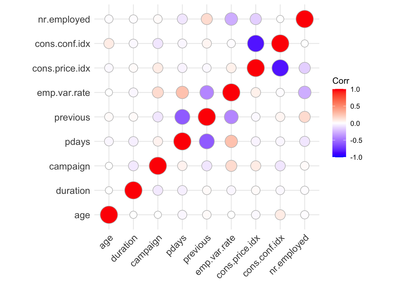

correlations = data_bank_marketing.select_dtypes(include=np.number).corr(method='pearson')
with pd.option_context('display.max_columns', 40):
  print(correlations)

                     age  duration  campaign     pdays  previous  emp.var.rate  cons.price.idx  cons.conf.idx  euribor3m  nr.employed
age             1.000000 -0.000866  0.004594 -0.034369  0.024365     -0.000371        0.000857       0.129372   0.010767    -0.017725
duration       -0.000866  1.000000 -0.071699 -0.047577  0.020640     -0.027968        0.005312      -0.008173  -0.032897    -0.044703
campaign        0.004594 -0.071699  1.000000  0.052584 -0.079141      0.150754        0.127836      -0.013733   0.135133     0.144095
pdays          -0.034369 -0.047577  0.052584  1.000000 -0.587514      0.271004        0.078889      -0.091342   0.296899     0.372605
previous        0.024365  0.020640 -0.079141 -0.587514  1.000000     -0.420489       -0.203130      -0.050936  -0.454494    -0.501333
emp.var.rate   -0.000371 -0.027968  0.150754  0.271004 -0.420489      1.000000        0.775334       0.196041   0.972245     0.906970
cons.price.idx  0.000857  0.005312  0.127836  0.078889 -0.203130      0.775334        1.000000       0.058986   0.688230     0.522034
cons.conf.idx   0.129372 -0.008173 -0.013733 -0.091342 -0.050936      0.196041        0.058986       1.000000   0.277686     0.100513
euribor3m       0.010767 -0.032897  0.135133  0.296899 -0.454494      0.972245        0.688230       0.277686   1.000000     0.945154
nr.employed    -0.017725 -0.044703  0.144095  0.372605 -0.501333      0.906970        0.522034       0.100513   0.945154     1.000000

names = data_bank_marketing.select_dtypes(include=np.number).columns.values.tolist()
hmap=sns.heatmap(correlations, 
        xticklabels=correlations.columns,
        yticklabels=correlations.columns)
hmap.xaxis.tick_top()
plt.xticks(rotation=30)

(array([0.5, 1.5, 2.5, 3.5, 4.5, 5.5, 6.5, 7.5, 8.5, 9.5]), [Text(0.5, 1, 'age'), Text(1.5, 1, 'duration'), Text(2.5, 1, 'campaign'), Text(3.5, 1, 'pdays'), Text(4.5, 1, 'previous'), Text(5.5, 1, 'emp.var.rate'), Text(6.5, 1, 'cons.price.idx'), Text(7.5, 1, 'cons.conf.idx'), Text(8.5, 1, 'euribor3m'), Text(9.5, 1, 'nr.employed')])

plt.show()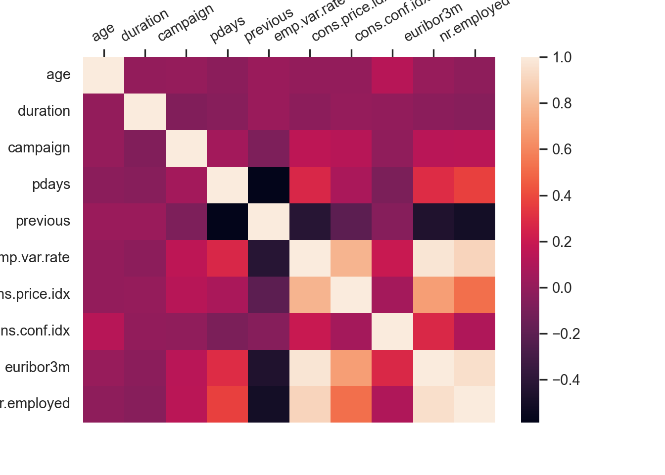

function cor_df(df::DataFrame)
  numeric_cols = names(df, Real)
  M=Matrix(data[!,numeric_cols])
  C=cor(M)
  cols=reshape(numeric_cols, 1, (length(numeric_cols)))
  
  (n,m) = size(C)
  hm=heatmap(C, fc=cgrad([:white,:dodgerblue4]), xticks=(1:m,numeric_cols), xrot=90, yticks=(1:m,numeric_cols), yflip=true, show = true)
  annotate!([(j, i, text(round(C[i,j],digits=3), 8,"Computer Modern",:black)) for i in 1:n for j in 1:m])
  
  return (hm, DataFrame(vcat(cols,C), :auto))
end

cor_df (generic function with 1 method)


hm,corr=cor_df(data)

(Plot{Plots.GRBackend() n=1}, 11×10 DataFrame
 Row │ x1            x2            x3          x4          x5          x6      ⋯
     │ Any           Any           Any         Any         Any         Any     ⋯
─────┼──────────────────────────────────────────────────────────────────────────
   1 │ age           duration      campaign    pdays       previous    emp.var ⋯
   2 │ 1.0           -0.000865705  0.00459358  -0.034369   0.0243647   -0.0003
   3 │ -0.000865705  1.0           -0.0716992  -0.047577   0.0206404   -0.0279
   4 │ 0.00459358    -0.0716992    1.0         0.0525836   -0.0791415  0.15075
   5 │ -0.034369     -0.047577     0.0525836   1.0         -0.587514   0.27100 ⋯
   6 │ 0.0243647     0.0206404     -0.0791415  -0.587514   1.0         -0.4204
   7 │ -0.000370685  -0.0279679    0.150754    0.271004    -0.420489   1.0
   8 │ 0.000856715   0.00531227    0.127836    0.0788891   -0.20313    0.77533
   9 │ 0.129372      -0.00817287   -0.0137331  -0.0913424  -0.0509364  0.19604 ⋯
  10 │ 0.0107674     -0.0328967    0.135133    0.296899    -0.454494   0.97224
  11 │ -0.0177251    -0.0447032    0.144095    0.372605    -0.501333   0.90697
                                                               5 columns omitted)

display(hm)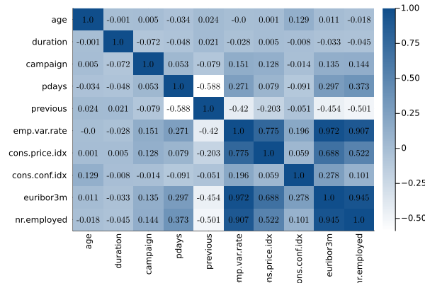

Observations

There is a negative correlation between cons.conf.idx and cons.price.idx

Category-wise percentage proportions of outcome

#https://stackoverflow.com/questions/24901061/in-r-how-do-i-compute-factors-percentage-given-on-different-variable


get_proportions = function(data, attribute, outcome, asPercent = TRUE) {
  
  multiplier = 1
  if (asPercent) {
    multiplier = 100
  }
  
  prop_df = rownames_to_column(multiplier*as.data.frame.matrix(prop.table(table(data %>% select(attribute,outcome)), 1))) %>% as_tibble() #%>% rename(attribute = rowname) %>% as_tibble()
  freq_df = as_tibble(multiplier*prop.table(table(data %>% select(attribute))))
  final_df = left_join(prop_df, freq_df, by = c(rowname = attribute))
}

knitr::kable(get_proportions(data_bank_marketing, 'job', 'y') %>% rename(job = rowname) %>% rename(overall = n) %>%  arrange(desc(yes)))

job	no	yes	overall
student	68.57143	31.428571	2.1244052
retired	74.76744	25.232558	4.1759736
unemployed	85.79882	14.201183	2.4618821
admin.	87.02744	12.972558	25.3034865
management	88.78249	11.217510	7.0991551
unknown	88.78788	11.212121	0.8012042
technician	89.17396	10.826042	16.3712732
self-employed	89.51443	10.485573	3.4500340
housemaid	90.00000	10.000000	2.5735651
entrepreneur	91.48352	8.516483	3.5350102
services	91.86193	8.138070	9.6363018
blue-collar	93.10568	6.894316	22.4677090

knitr::kable(get_proportions(data_bank_marketing, 'education', 'y') %>% rename(education = rowname) %>% rename(overall = n) %>% arrange(desc(yes)))

education	no	yes	overall
illiterate	77.77778	22.222222	0.043702
unknown	85.49971	14.500289	4.202680
university.degree	86.27548	13.724523	29.542585
professional.course	88.65154	11.348465	12.729436
high.school	89.16448	10.835523	23.101389
basic.4y	89.75096	10.249042	10.138875
basic.6y	91.79756	8.202443	5.564728
basic.9y	92.17535	7.824649	14.676605

knitr::kable(get_proportions(data_bank_marketing, 'marital', 'y') %>% rename(marital = rowname) %>% rename(overall = n) %>% arrange(desc(yes)))

marital	no	yes	overall
unknown	85.00000	15.00000	0.1942313
single	85.99585	14.00415	28.0858502
divorced	89.67910	10.32090	11.1974361
married	89.84275	10.15725	60.5224823

knitr::kable(get_proportions(data_bank_marketing, 'default', 'y') %>% rename(default = rowname) %>% rename(overall = n) %>% arrange(desc(yes)))

default	no	yes	overall
no	87.12103	12.87897	79.1201321
unknown	94.84704	5.15296	20.8725842
yes	100.00000	0.00000	0.0072837

knitr::kable(get_proportions(data_bank_marketing, 'housing', 'y') %>% rename(housing = rowname) %>% rename(overall = n) %>% arrange(desc(yes)))

housing	no	yes	overall
yes	88.38061	11.61939	52.384190
no	89.12040	10.87960	45.212198
unknown	89.19192	10.80808	2.403613

knitr::kable(get_proportions(data_bank_marketing, 'loan', 'y') %>% rename(loan = rowname) %>% rename(overall = n) %>% arrange(desc(yes)))

loan	no	yes	overall
no	88.65979	11.34021	82.426920
yes	89.06850	10.93150	15.169467
unknown	89.19192	10.80808	2.403613

knitr::kable(get_proportions(data_bank_marketing, 'contact', 'y') %>% rename(contact = rowname) %>% rename(overall = n) %>% arrange(desc(yes)))

contact	no	yes	overall
cellular	85.26239	14.737607	63.4748
telephone	94.76868	5.231321	36.5252

knitr::kable(get_proportions(data_bank_marketing, 'month', 'y') %>% rename(month = rowname) %>% rename(overall = n) %>% arrange(desc(yes)))

month	no	yes	overall
mar	49.45055	50.549450	1.3256288
dec	51.09890	48.901099	0.4418763
sep	55.08772	44.912281	1.3838982
oct	56.12813	43.871866	1.7432262
apr	79.52128	20.478723	6.3902107
aug	89.39786	10.602137	14.9995144
jun	89.48853	10.511470	12.9115276
nov	89.85613	10.143867	9.9567835
jul	90.95344	9.046557	17.4176945
may	93.56526	6.434745	33.4296397

knitr::kable(get_proportions(data_bank_marketing, 'poutcome', 'y') %>% rename(poutcome = rowname) %>% rename(overall = n) %>% arrange(desc(yes)))

poutcome	no	yes	overall
success	34.88711	65.112892	3.333495
failure	85.77140	14.228598	10.323395
nonexistent	91.16779	8.832213	86.343110

knitr::kable(get_proportions(data_bank_marketing, 'day_of_week', 'y') %>% rename(day_of_week = rowname) %>% rename(overall = n) %>% arrange(desc(yes)))

day_of_week	no	yes	overall
thu	87.88125	12.11875	20.93571
tue	88.22002	11.77998	19.64164
wed	88.33292	11.66708	19.74847
fri	89.19126	10.80874	19.00311
mon	90.05168	9.94832	20.67107


def get_proportions(df, category, outcome):
  df=data_bank_marketing[[category,outcome]].groupby(category).value_counts(normalize=True).mul(100)
  df_overall=data_bank_marketing[[category]].groupby(category)
  df_overall=(df_overall.value_counts()/sum(df_overall.value_counts())).mul(100)
  df_overall=pd.DataFrame(df_overall).reset_index()
  df_overall=df_overall.rename(columns={0:'overall'})
  df_yes=df.iloc[1::2]
  df_yes=pd.DataFrame(df_yes).reset_index().drop([outcome], axis = 1)
  df_yes=df_yes.rename(columns={0:'yes'})
  
  df_no=df.iloc[::2]
  df_no=pd.DataFrame(df_no).reset_index().drop([outcome], axis = 1)
  df_no=df_no.rename(columns={0:'no'})
  
  final_df = df_no.join(df_yes['yes'])
  final_df = final_df.join(df_overall['overall']).sort_values('yes', ascending=False)
  return final_df
  
proportions=get_proportions(data_bank_marketing,'job', 'y')
dsp.Markdown(proportions.to_markdown(index=False))

job	no	yes	overall
student	68.5714	31.4286	2.12441
retired	74.7674	25.2326	4.17597
unemployed	85.7988	14.2012	2.46188
admin.	87.0274	12.9726	25.3035
management	88.7825	11.2175	7.09916
unknown	88.7879	11.2121	0.801204
technician	89.174	10.826	16.3713
self-employed	89.5144	10.4856	3.45003
housemaid	90	10	2.57357
entrepreneur	91.4835	8.51648	3.53501
services	91.8619	8.13807	9.6363
blue-collar	93.1057	6.89432	22.4677

proportions=get_proportions(data_bank_marketing,'education', 'y')  
dsp.Markdown(proportions.to_markdown(index=False))

education	no	yes	overall
illiterate	77.7778	22.2222	0.043702
unknown	85.4997	14.5003	4.20268
university.degree	86.2755	13.7245	29.5426
professional.course	88.6515	11.3485	12.7294
high.school	89.1645	10.8355	23.1014
basic.4y	89.751	10.249	10.1389
basic.6y	91.7976	8.20244	5.56473
basic.9y	92.1754	7.82465	14.6766

proportions=get_proportions(data_bank_marketing, 'marital', 'y')
dsp.Markdown(proportions.to_markdown(index=False))

marital	no	yes	overall
unknown	85	15	0.194231
single	85.9959	14.0041	28.0859
divorced	89.6791	10.3209	11.1974
married	89.8427	10.1573	60.5225

proportions=get_proportions(data_bank_marketing, 'default', 'y')
dsp.Markdown(proportions.to_markdown(index=False))

default	no	yes	overall
no	87.121	12.879	79.1201
unknown	94.847	5.15296	20.8726
yes	100	nan	0.00728367

proportions=get_proportions(data_bank_marketing, 'housing', 'y')
dsp.Markdown(proportions.to_markdown(index=False))

housing	no	yes	overall
yes	88.3806	11.6194	52.3842
no	89.1204	10.8796	45.2122
unknown	89.1919	10.8081	2.40361

proportions=get_proportions(data_bank_marketing, 'loan', 'y')
dsp.Markdown(proportions.to_markdown(index=False))

loan	no	yes	overall
no	88.6598	11.3402	82.4269
yes	89.0685	10.9315	15.1695
unknown	89.1919	10.8081	2.40361

proportions=get_proportions(data_bank_marketing, 'contact', 'y')
dsp.Markdown(proportions.to_markdown(index=False))

contact	no	yes	overall
cellular	85.2624	14.7376	63.4748
telephone	94.7687	5.23132	36.5252

proportions=get_proportions(data_bank_marketing, 'month', 'y')
dsp.Markdown(proportions.to_markdown(index=False))

month	no	yes	overall
mar	50.5495	49.4505	1.32563
dec	51.0989	48.9011	0.441876
sep	55.0877	44.9123	1.3839
oct	56.1281	43.8719	1.74323
apr	79.5213	20.4787	6.39021
aug	89.3979	10.6021	14.9995
jun	89.4885	10.5115	12.9115
nov	89.8561	10.1439	9.95678
jul	90.9534	9.04656	17.4177
may	93.5653	6.43474	33.4296

proportions=get_proportions(data_bank_marketing, 'poutcome', 'y')
dsp.Markdown(proportions.to_markdown(index=False))

poutcome	no	yes	overall
success	65.1129	34.8871	3.3335
failure	85.7714	14.2286	10.3234
nonexistent	91.1678	8.83221	86.3431

proportions=get_proportions(data_bank_marketing, 'day_of_week', 'y')
dsp.Markdown(proportions.to_markdown(index=False))

day_of_week	no	yes	overall
thu	87.8812	12.1188	20.9357
tue	88.22	11.78	19.6416
wed	88.3329	11.6671	19.7485
fri	89.1913	10.8087	19.0031
mon	90.0517	9.94832	20.6711

function get_proportions(df::DataFrame, category::String, outcome::String, filter_str::String)
  gdf_outcome = groupby(df, [category, outcome])
  D = DataFrame(combine(gdf_outcome, nrow))
  
  counts_1=@chain D begin
    filter(outcome => isequal(filter_str), _)
    select(:nrow)
  end
  
  counts_2=@chain D begin
    filter(outcome => !isequal(filter_str), _)
    select(:nrow)
  end
  
  if nrow(counts_1) != nrow(counts_2)
    diff = nrow(counts_1) - nrow(counts_2)
    U = counts_1
    if diff > 0 #counts_1 has more rows
      U = counts_2
    end
    
    i=0
    while i < abs(diff)
      push!(U, [0])
      i += 1
    end
    
  end
  
  rename!(counts_1, :nrow=>:yes)
  rename!(counts_2, :nrow=>:no)
  
  counts=DataFrame(hcat(counts_1,counts_2))
  
  @transform!(counts, :all = :yes .+ :no)
  @transform!(counts, :prop = :yes ./ :all)
  @transform!(counts, :overall = :all ./ nrow(df))
  
  counts.prop .*= 100
  counts.overall .*= 100
  
  N = unique(select(D, category))
  
  sort!(hcat(N,select(counts,[:prop,:overall])), :prop, rev=true)
end

get_proportions (generic function with 1 method)


get_proportions(data, "job", "y", "yes")

12×3 DataFrame
 Row │ job            prop      overall
     │ String15       Float64   Float64
─────┼────────────────────────────────────
   1 │ student        31.4286    2.12441
   2 │ retired        25.2326    4.17597
   3 │ unemployed     14.2012    2.46188
   4 │ admin.         12.9726   25.3035
   5 │ management     11.2175    7.09916
   6 │ unknown        11.2121    0.801204
   7 │ technician     10.826    16.3713
   8 │ self-employed  10.4856    3.45003
   9 │ housemaid      10.0       2.57357
  10 │ entrepreneur    8.51648   3.53501
  11 │ services        8.13807   9.6363
  12 │ blue-collar     6.89432  22.4677

get_proportions(data, "education", "y", "yes")

8×3 DataFrame
 Row │ education            prop      overall
     │ String31             Float64   Float64
─────┼──────────────────────────────────────────
   1 │ illiterate           22.2222    0.043702
   2 │ unknown              14.5003    4.20268
   3 │ university.degree    13.7245   29.5426
   4 │ professional.course  11.3485   12.7294
   5 │ high.school          10.8355   23.1014
   6 │ basic.4y             10.249    10.1389
   7 │ basic.6y              8.20244   5.56473
   8 │ basic.9y              7.82465  14.6766

get_proportions(data, "marital", "y", "yes")

4×3 DataFrame
 Row │ marital   prop     overall
     │ String15  Float64  Float64
─────┼──────────────────────────────
   1 │ unknown   15.0      0.194231
   2 │ single    14.0041  28.0859
   3 │ divorced  10.3209  11.1974
   4 │ married   10.1573  60.5225

get_proportions(data, "default", "y", "yes")

3×3 DataFrame
 Row │ default  prop      overall
     │ String7  Float64   Float64
─────┼────────────────────────────────
   1 │ no       12.879    79.1201
   2 │ unknown   5.15296  20.8726
   3 │ yes       0.0       0.00728367

get_proportions(data, "housing", "y", "yes")

3×3 DataFrame
 Row │ housing  prop     overall
     │ String7  Float64  Float64
─────┼────────────────────────────
   1 │ yes      11.6194  52.3842
   2 │ no       10.8796  45.2122
   3 │ unknown  10.8081   2.40361

get_proportions(data, "loan", "y", "yes")

3×3 DataFrame
 Row │ loan     prop     overall
     │ String7  Float64  Float64
─────┼────────────────────────────
   1 │ no       11.3402  82.4269
   2 │ yes      10.9315  15.1695
   3 │ unknown  10.8081   2.40361

get_proportions(data, "contact", "y", "yes")

2×3 DataFrame
 Row │ contact    prop      overall
     │ String15   Float64   Float64
─────┼──────────────────────────────
   1 │ cellular   14.7376   63.4748
   2 │ telephone   5.23132  36.5252

get_proportions(data, "month", "y", "yes")

10×3 DataFrame
 Row │ month    prop      overall
     │ String3  Float64   Float64
─────┼──────────────────────────────
   1 │ mar      50.5495    1.32563
   2 │ dec      48.9011    0.441876
   3 │ sep      44.9123    1.3839
   4 │ oct      43.8719    1.74323
   5 │ apr      20.4787    6.39021
   6 │ aug      10.6021   14.9995
   7 │ jun      10.5115   12.9115
   8 │ nov      10.1439    9.95678
   9 │ jul       9.04656  17.4177
  10 │ may       6.43474  33.4296

Observations

job: There is higher percentage of yes outcome for students and retired persons, but the overall proportion of these categories is low. Perhaps a targeted campaign could be fruitful. Among the higher frequencies, admin has higher proportion of yes outcome.
education: There is higher percentage of yes outcome for illiterate - but this number can be ignored as the frequency of the category is negligible. Among the higher frequencies, university.degree has the highest positive outcome.
marital: unknown and single people have the highest positive outcome.
default: Very few people have credit defaults; none of those that do opt for the deposit
housing: Those having housing loans are slightly more likely to opt for the deposit; but the difference is only 1%
contact: Curiously, those contacted on cellular phones have a significantly higher possibility of subscribing to the deposit; this may be worth investigating further to determine causation.
month: For some reason, the months where there were much fewer calls have a much larger chance of subscribing for the loan. This definitely seems to be worthy of further investigation
day_of_week: Not a significant difference in outcome across the days of the week; though Thursdays have a slightly higher chance of positive outcome, and Mondays slightly lower.

Actions taken

Convert euribor3m values to numeric.

data_bank_marketing$euribor3m = as.numeric(data_bank_marketing$euribor3m)

Actions identified

Apply relevant transformations to reduce positive and negative skews in the data.

Numeric Attributes

Age

ggplot(data_bank_marketing) + geom_density(aes(x=(age), color=factor(y)))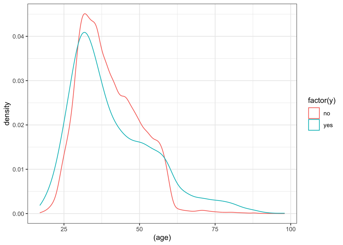

ggplot(data_bank_marketing) + geom_boxplot(aes(x=factor(y), y = age))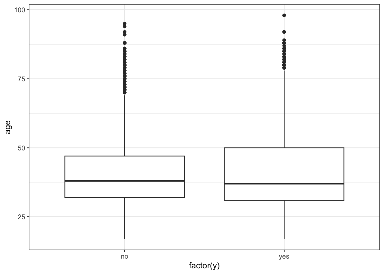

p = sns.displot(data_bank_marketing, x="age", hue="y", kind="kde", height = 5, aspect = 1.5)
plt.show()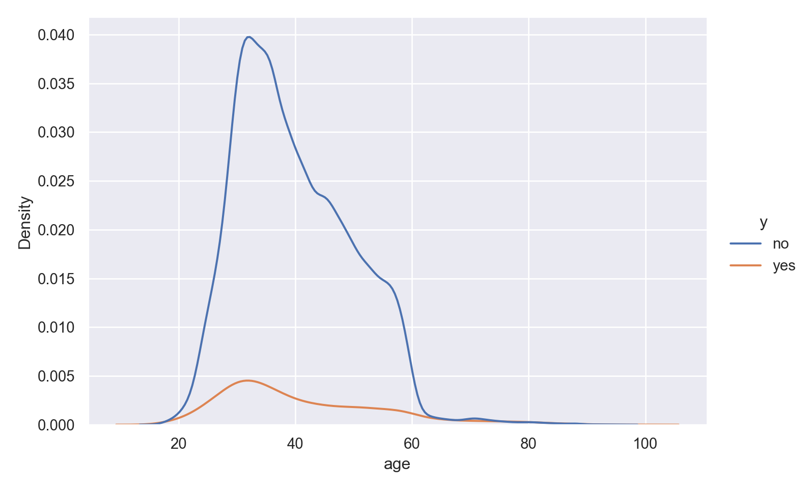

p = sns.catplot(data=data_bank_marketing, x="y", y="age", kind="box", height = 5, aspect = 1.5)
plt.show()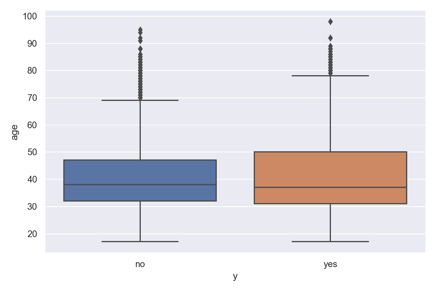

@df data density(:age, group = (:y))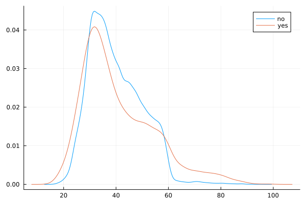

Observations

The data is right (positively) skewed, with more younger respondents.
The density curve indicates higher ‘yes’ outcome for age < 26 and age > 60, which was also seen in the numerical inspection.
The boxplot shows slightly more variation for ‘yes’ outcome, but median value of age is similar for both outcomes, with just a slightly lower age associated with ‘yes’ outcome.

duration

ggplot(data_bank_marketing) + geom_density(aes(x=(duration), color=factor(y)))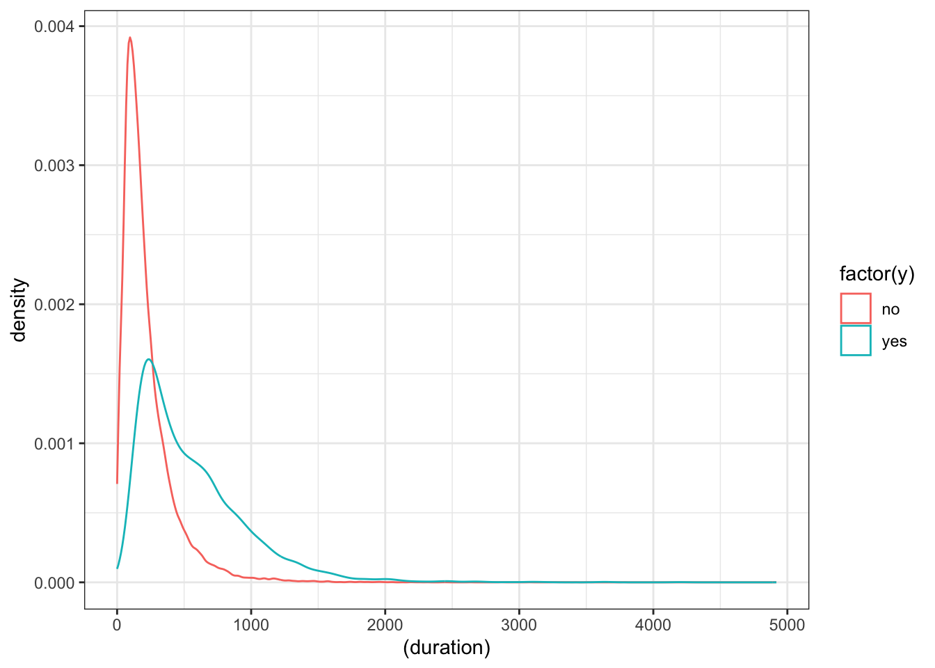

ggplot(data_bank_marketing) + geom_boxplot(aes(x=factor(y), y=duration))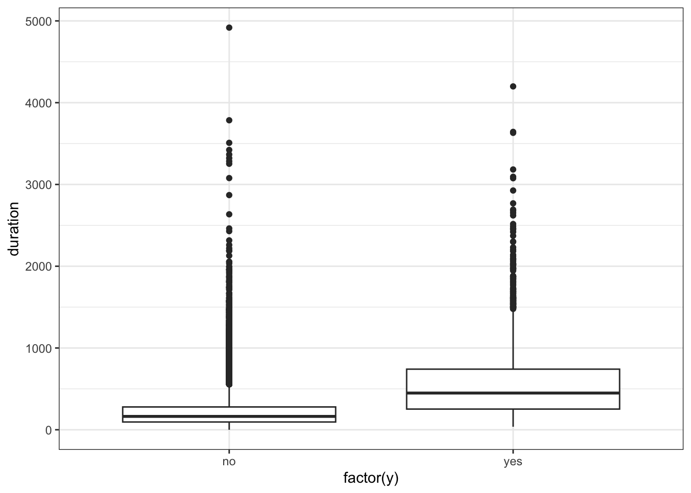

p=sns.displot(data_bank_marketing, x="duration", hue="y", kind="kde", height = 5, aspect = 1.5)
plt.show()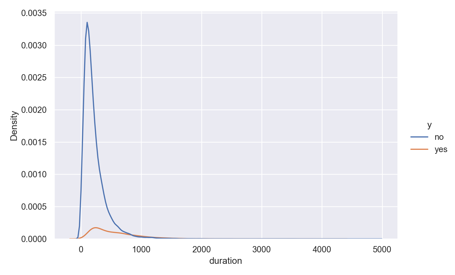

p=sns.catplot(data=data_bank_marketing, x="y", y="duration", kind="box", height = 5, aspect = 1.5)
plt.show()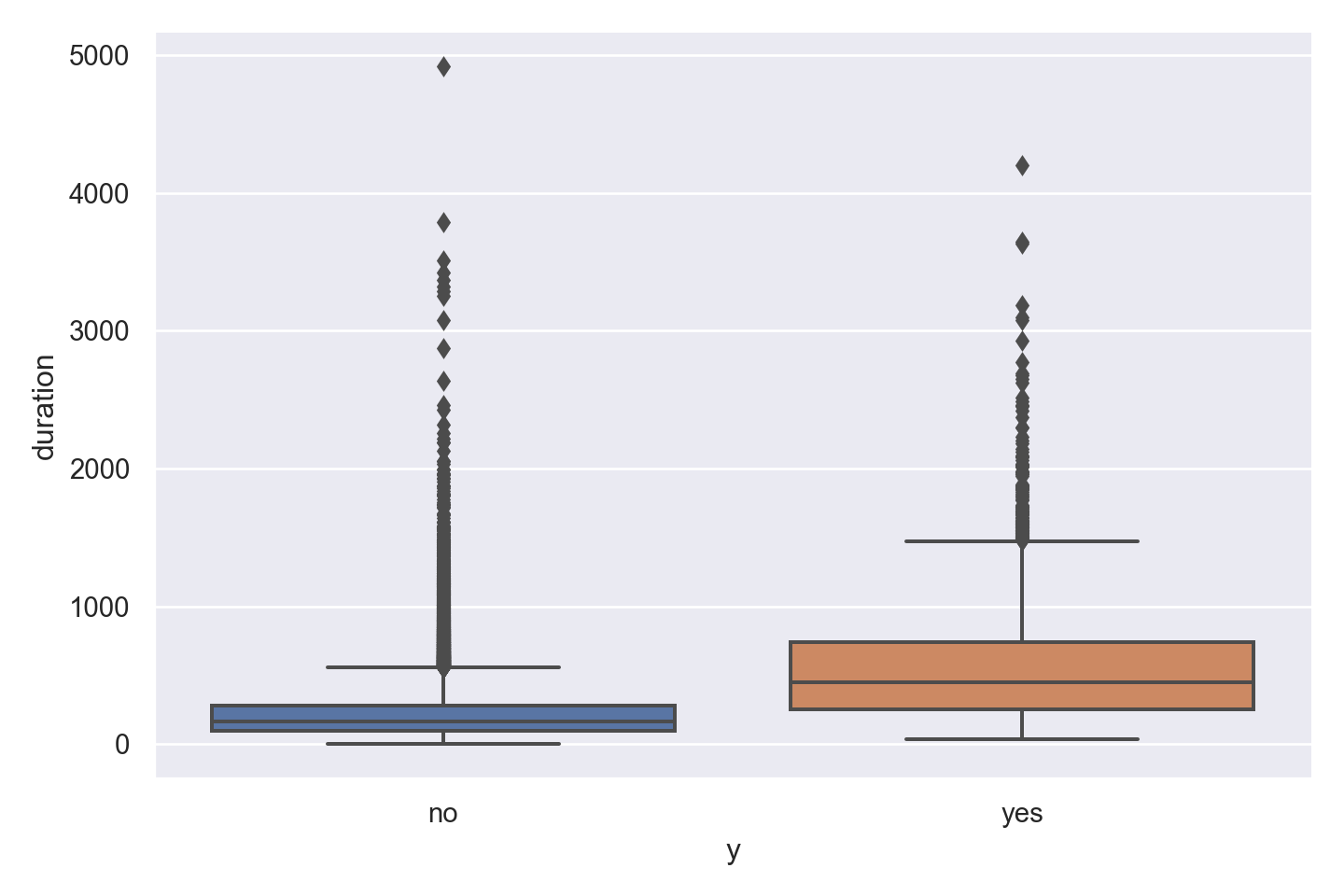

@df data density(:duration, group = (:y))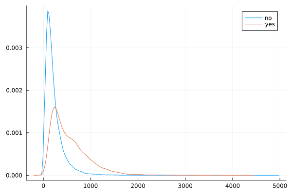

Observations

The data is heavily right (positively) skewed, towards low call duration.
As expected, the box plot indicates higher ‘yes’ outcome for higher duration, however as mentioned in the data dictionary, this will not help in predictive modelling as duration is not known before placing a call. It is the result of a ‘yes’ decision, and not its cause.

pdays

ggplot(data_bank_marketing) + geom_bar(aes(x=factor(pdays), fill=factor(y)))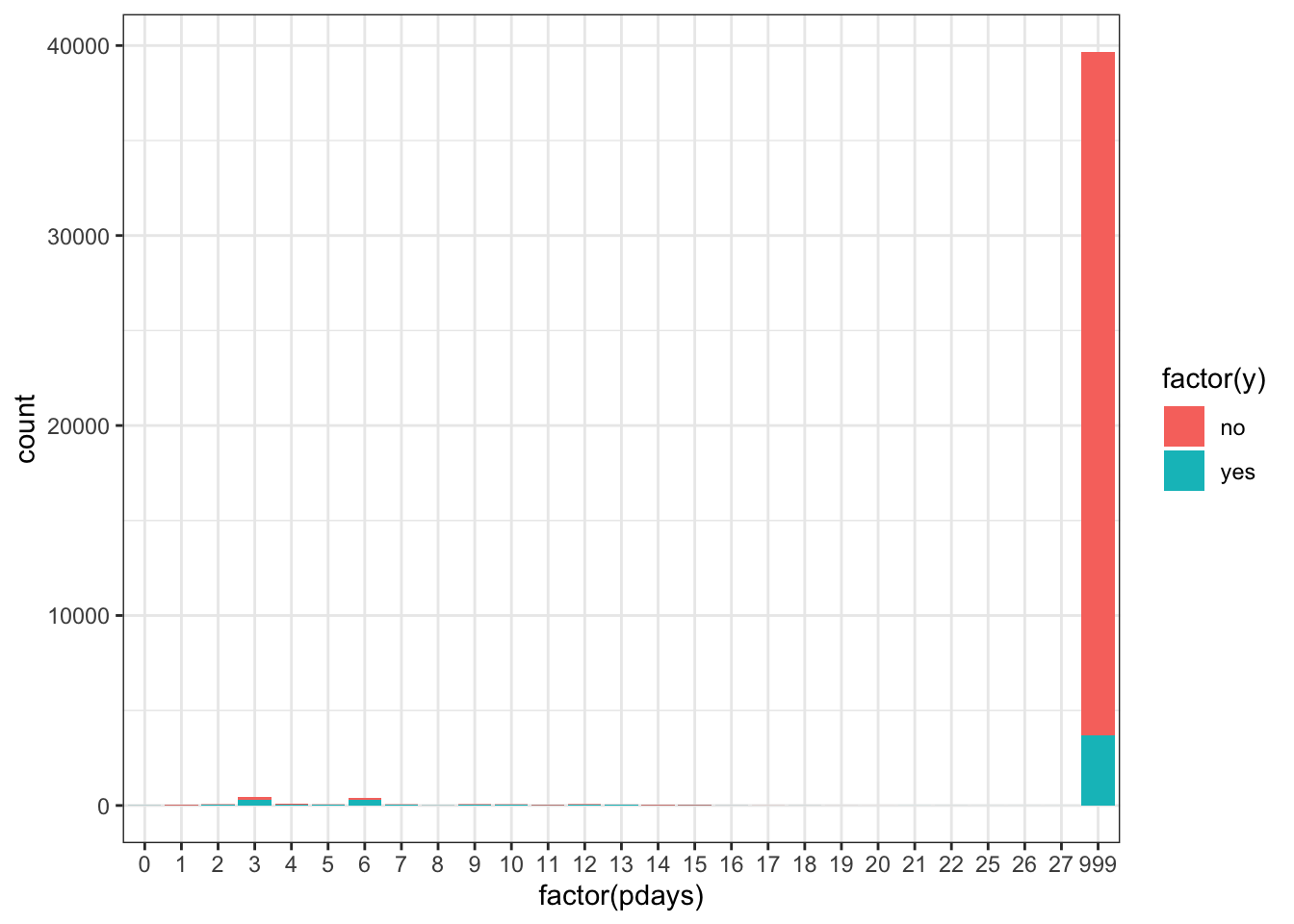

ggplot(data_bank_marketing  %>% filter(pdays<999)) + geom_density(aes(x=(pdays), color=factor(y)))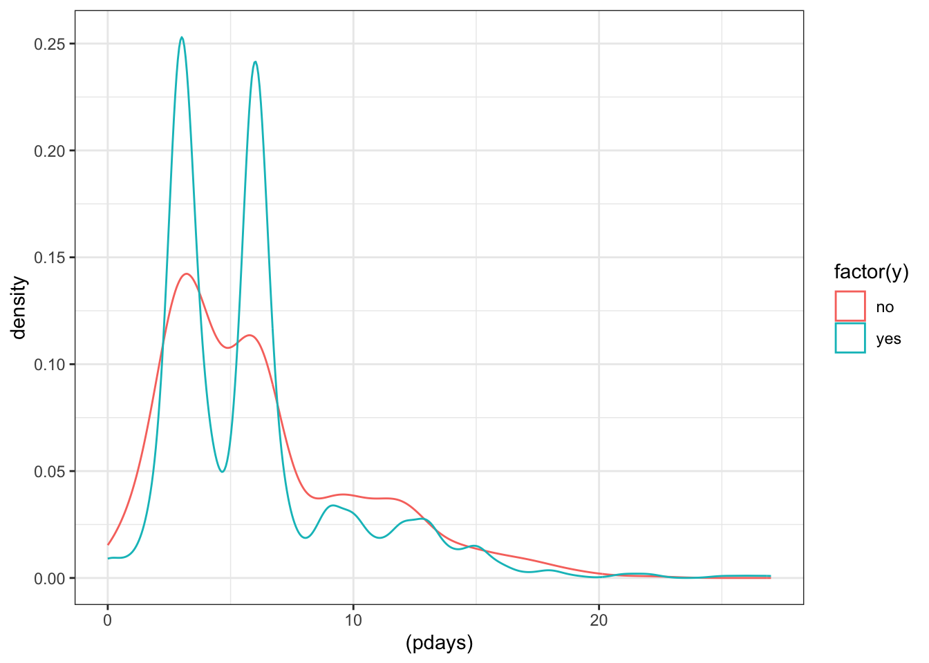

ggplot(data_bank_marketing %>% filter(pdays<999)) + geom_boxplot(aes(x=factor(y), y=pdays))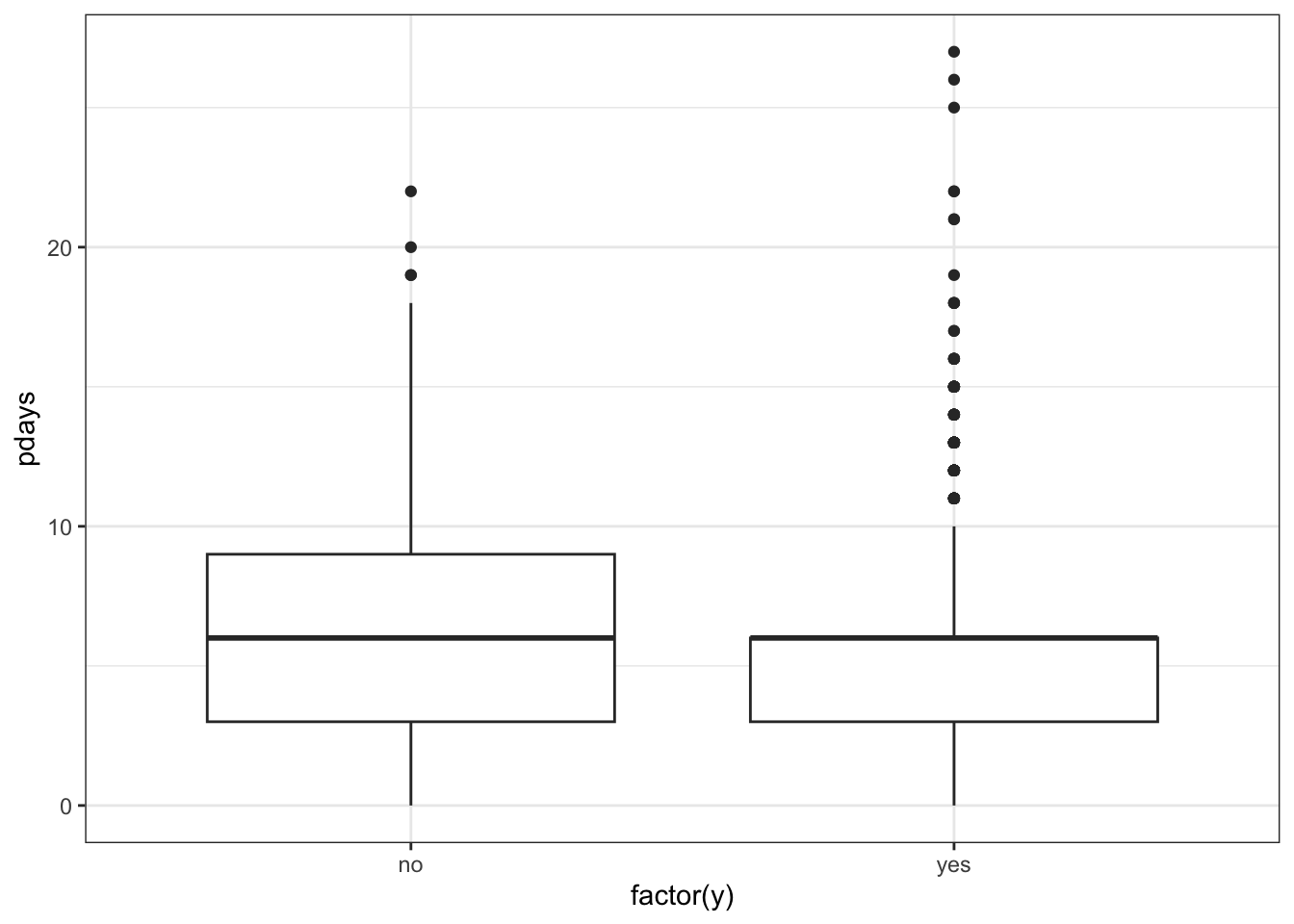

p=sns.catplot(data=data_bank_marketing, x="pdays", hue="y", kind="count", height = 5, aspect = 1.5)
plt.show()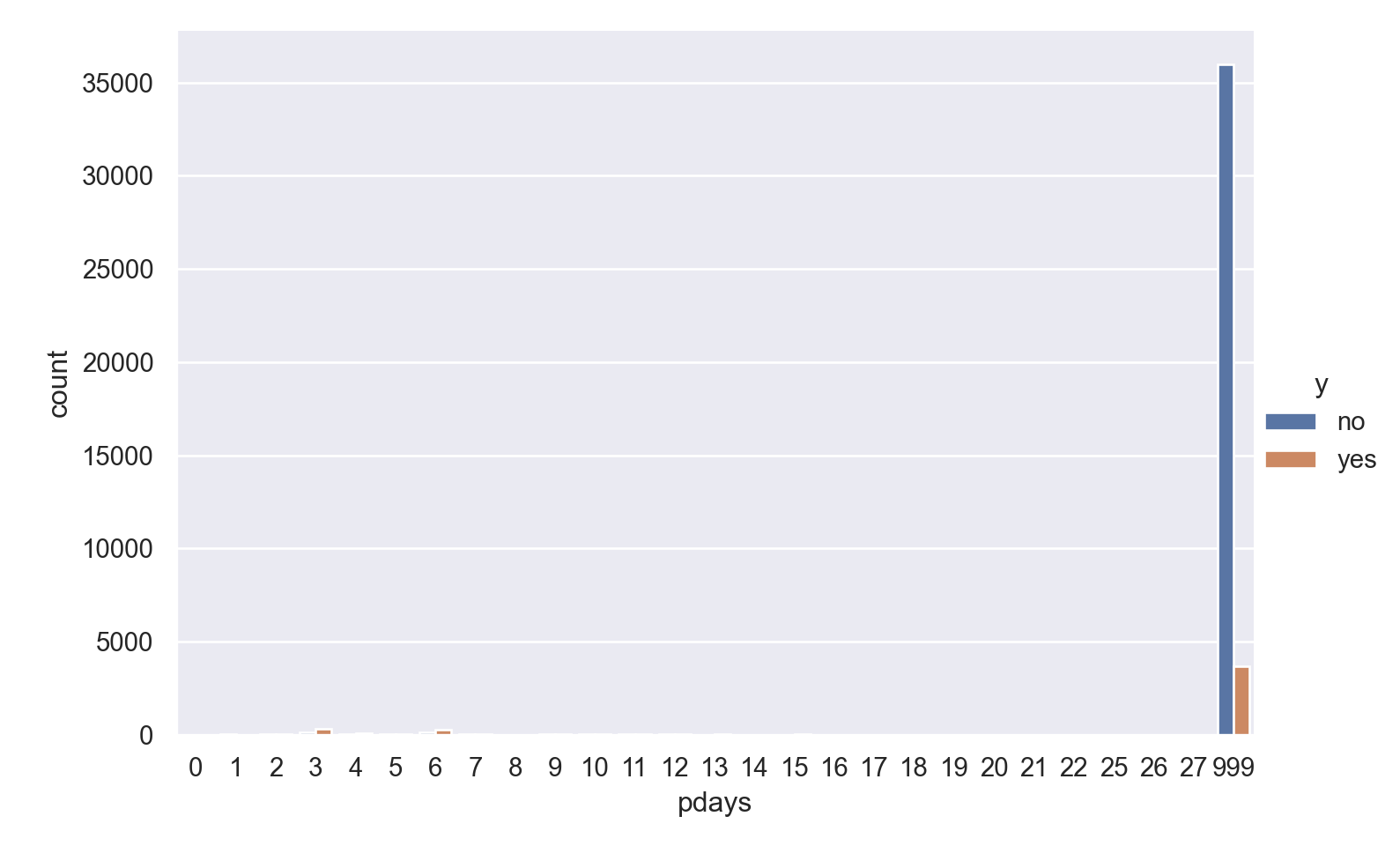

@df data density(:pdays, group = (:y))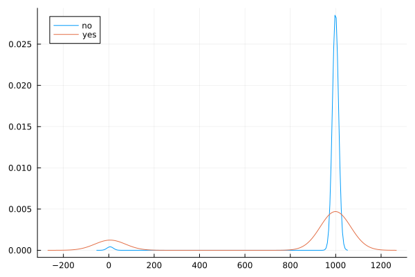

Observations

The vast majority of people were not previously contacted, so there is a very high left skew.
Filtering to only include the previously contacted people reveals a bi-modal pattern in the data, especially for respondents with ‘yes’ outcome.
For those that were previously contacted, median value of days since previous contact is the same for both outcomes, but ‘yes’ outcome has many outliers on the higher end.

ggplot(data_bank_marketing) + geom_bar(aes(x=factor(previous), fill=factor(y)))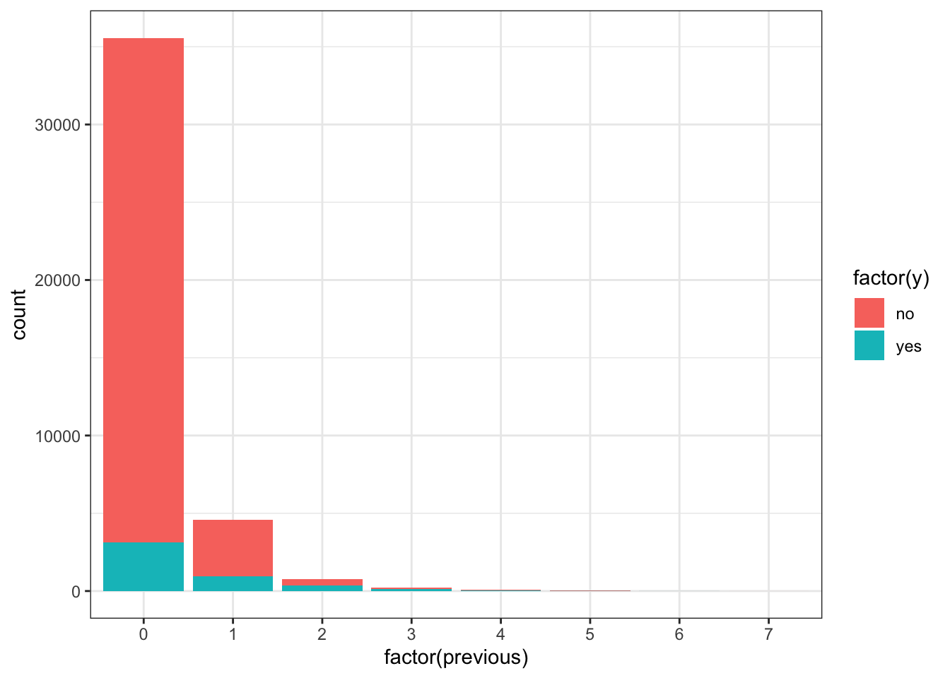

ggplot(data_bank_marketing) + geom_density(aes(x=previous, color=factor(y)))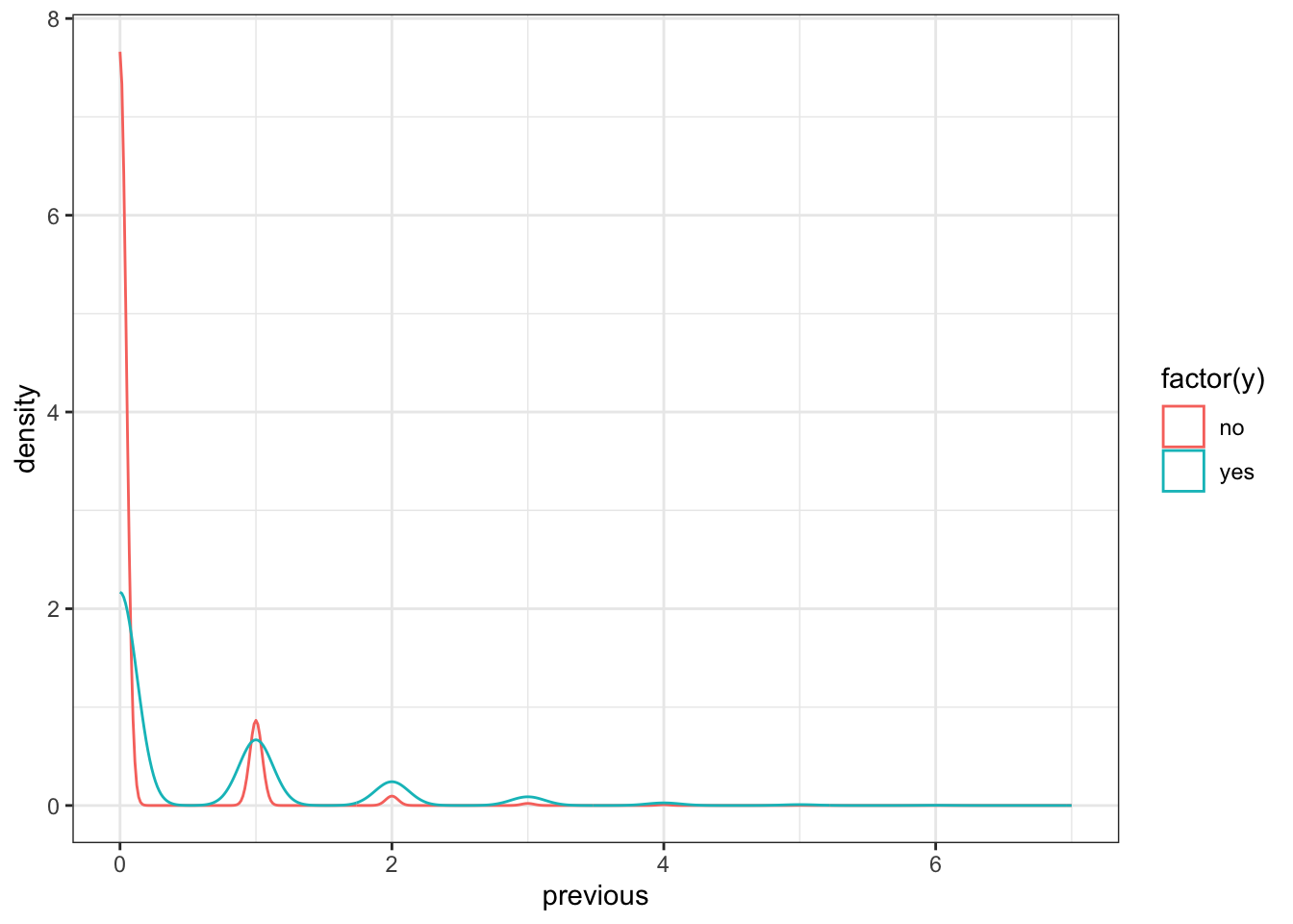

p=sns.catplot(data=data_bank_marketing, x="previous", hue="y", kind="count", height = 5, aspect = 1.5)
plt.show()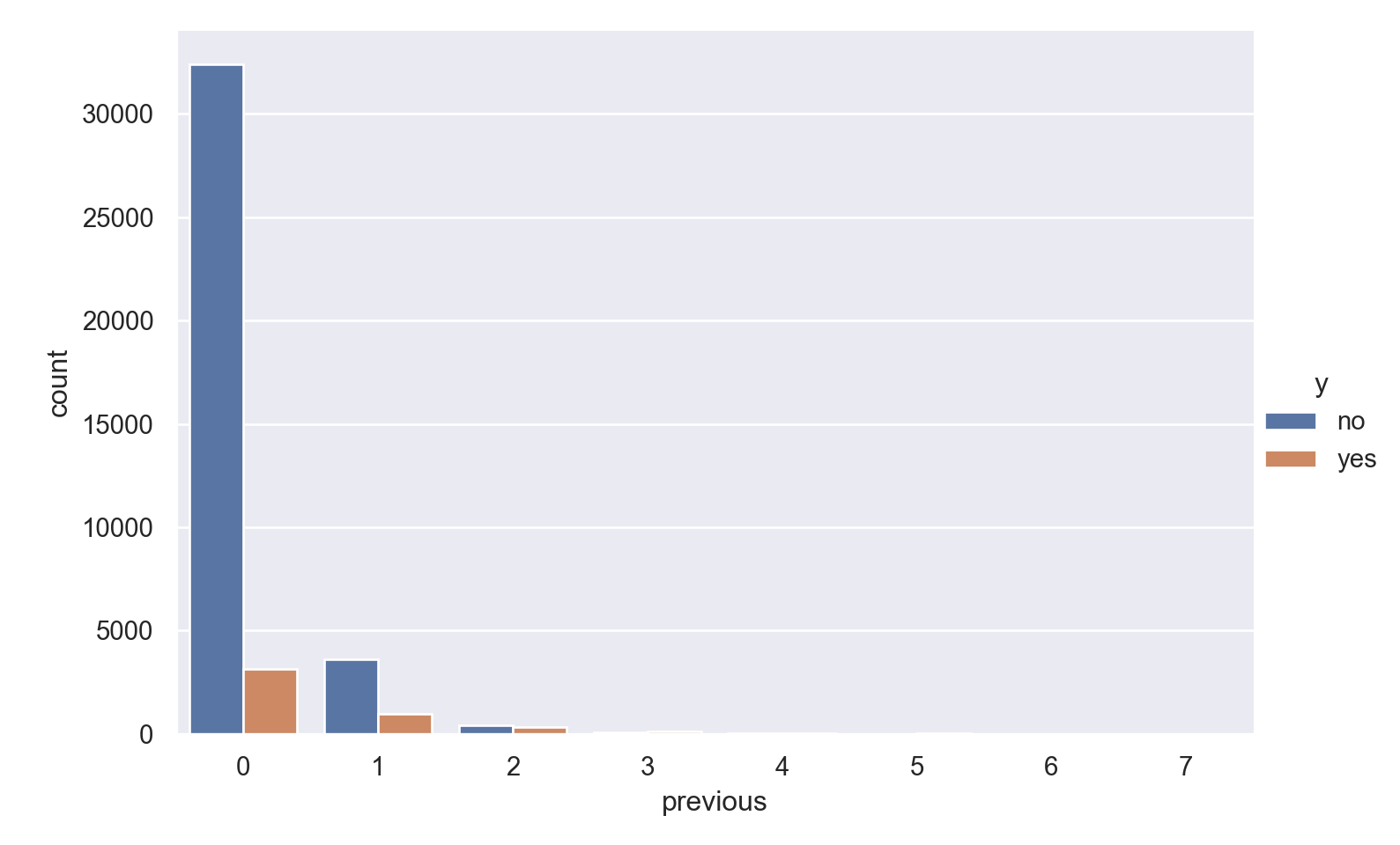

p=sns.displot(data_bank_marketing, x="previous", hue="y", kind="kde", height = 5, aspect = 1.5)
plt.show()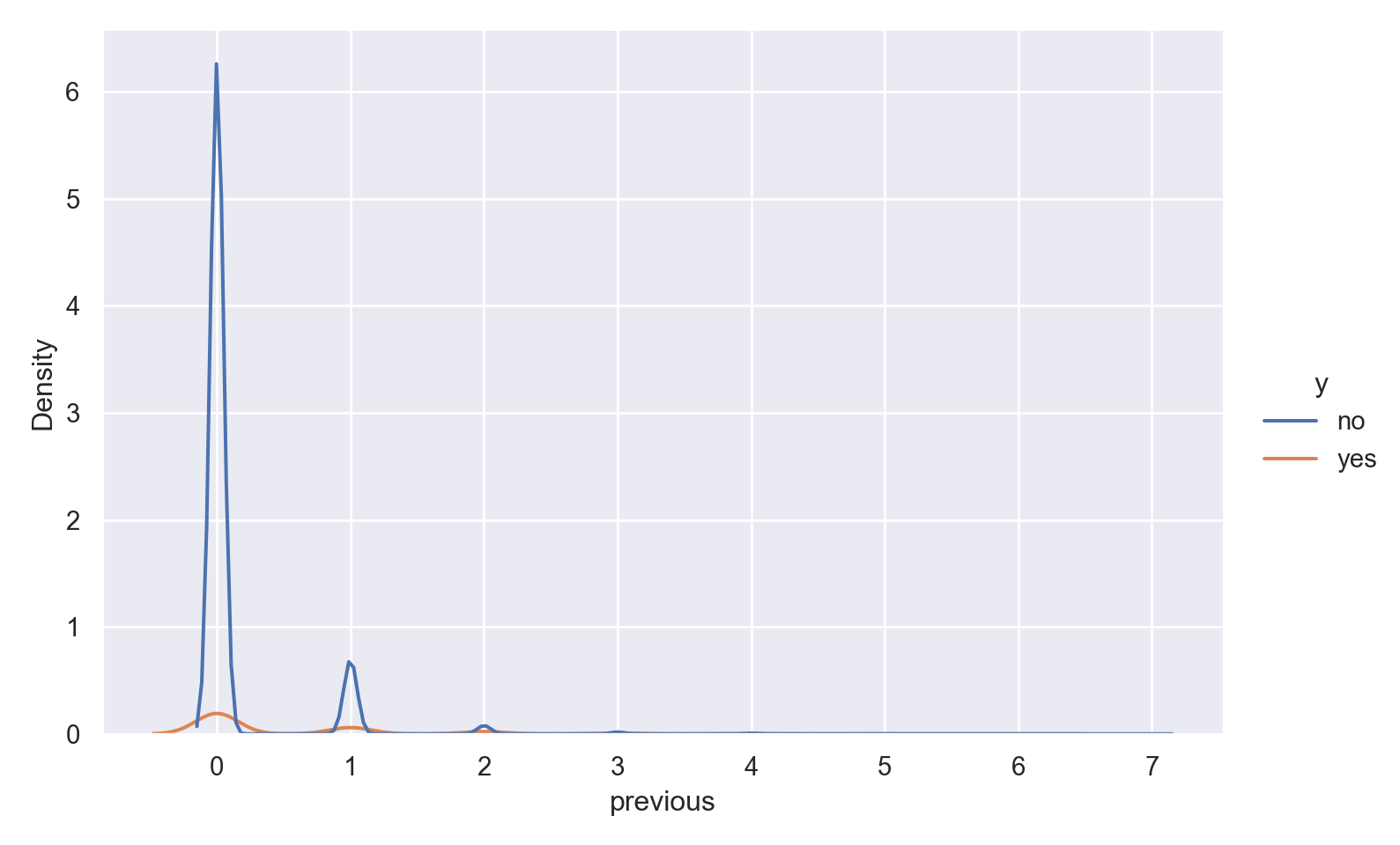

@df data density(:previous, group = (:y))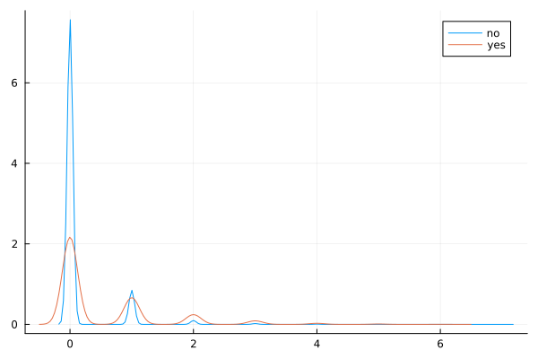

Observations

The vast majority of people were not previously contacted in the previous campaign, so there is a very high right skew.
The few people who were contacted multiple times seem to show higher ‘yes’ outcome for the current campaign.

campaign

ggplot(data_bank_marketing) + geom_density(aes(x=campaign, color=factor(y)))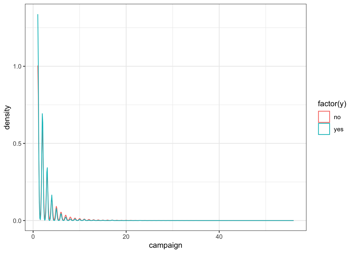

ggplot(data_bank_marketing) + geom_bar(aes(y=factor(campaign), fill=factor(y)))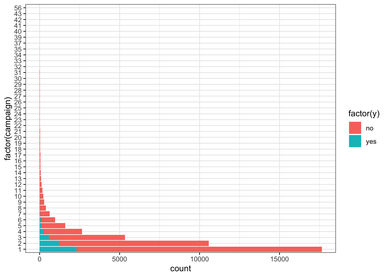

p=sns.displot(data_bank_marketing, x="campaign", hue="y", kind="kde", height = 5, aspect = 1.5)
plt.show()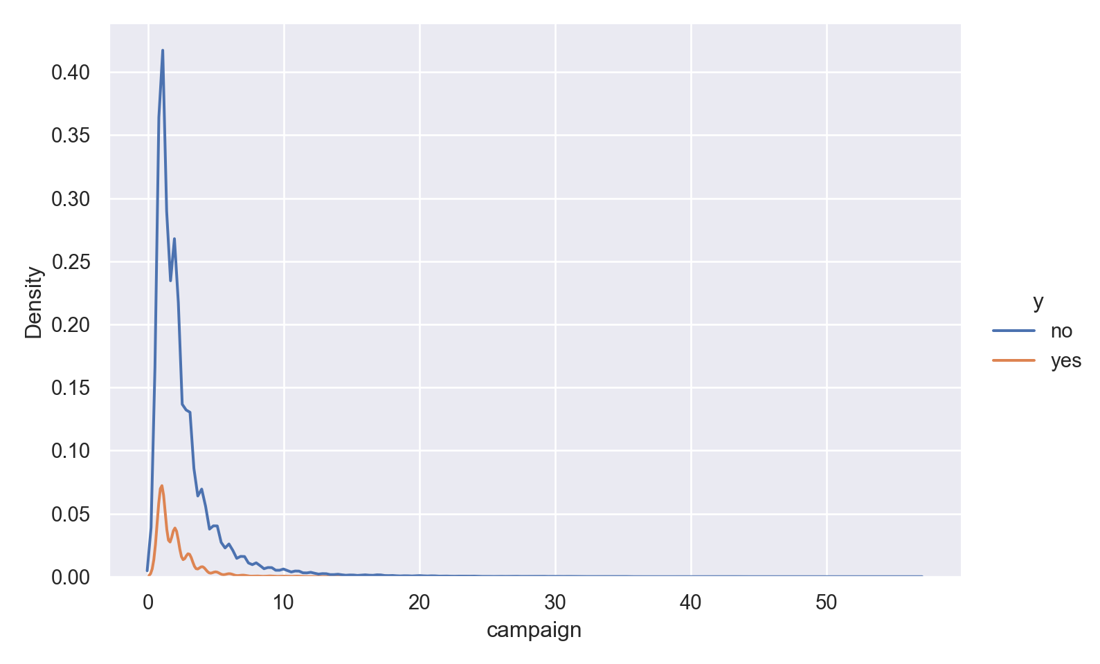

p=sns.catplot(data=data_bank_marketing, y="campaign", hue="y", kind="count", height = 5, aspect = 1.5)
plt.show()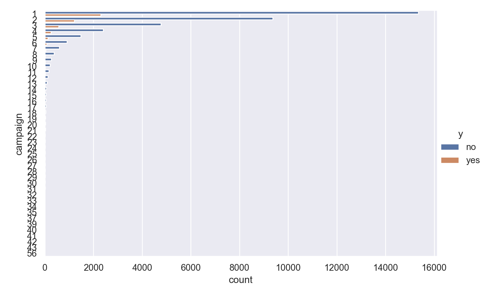

data1 = @transform(data, :campaign = categorical(:campaign));
p=@df data1 bar(:campaign, group = (:y))

Plot{Plots.GRBackend() n=2}

@df data1 density(:campaign, group = (:y))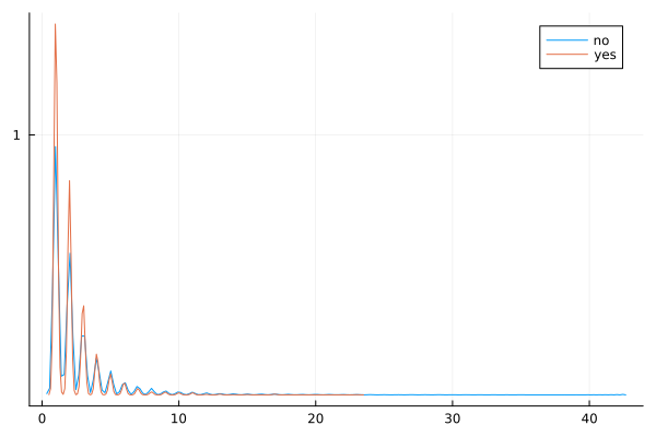

display(p)

Plot{Plots.GRBackend() n=2}

Observations

The vast majority of people were contacted only once in the current campaign, so there is a very high right skew.
The few people who were contacted multiple times seem to show higher ‘yes’ outcome.

emp.var.rate

ggplot(data_bank_marketing) + geom_density(aes(x=emp.var.rate, color=factor(y)))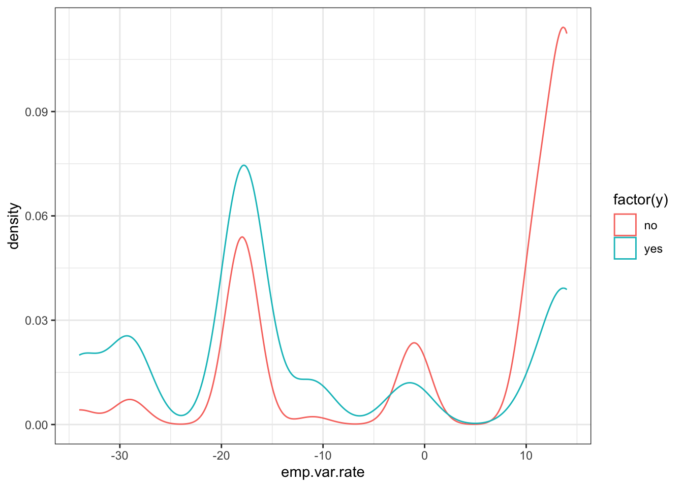

ggplot(data_bank_marketing) + geom_boxplot(aes(x=factor(y), y=emp.var.rate))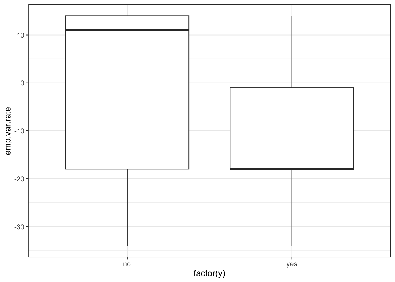

p=sns.displot(data_bank_marketing, x="emp.var.rate", hue="y", kind="kde", height = 5, aspect = 1.5)
plt.show()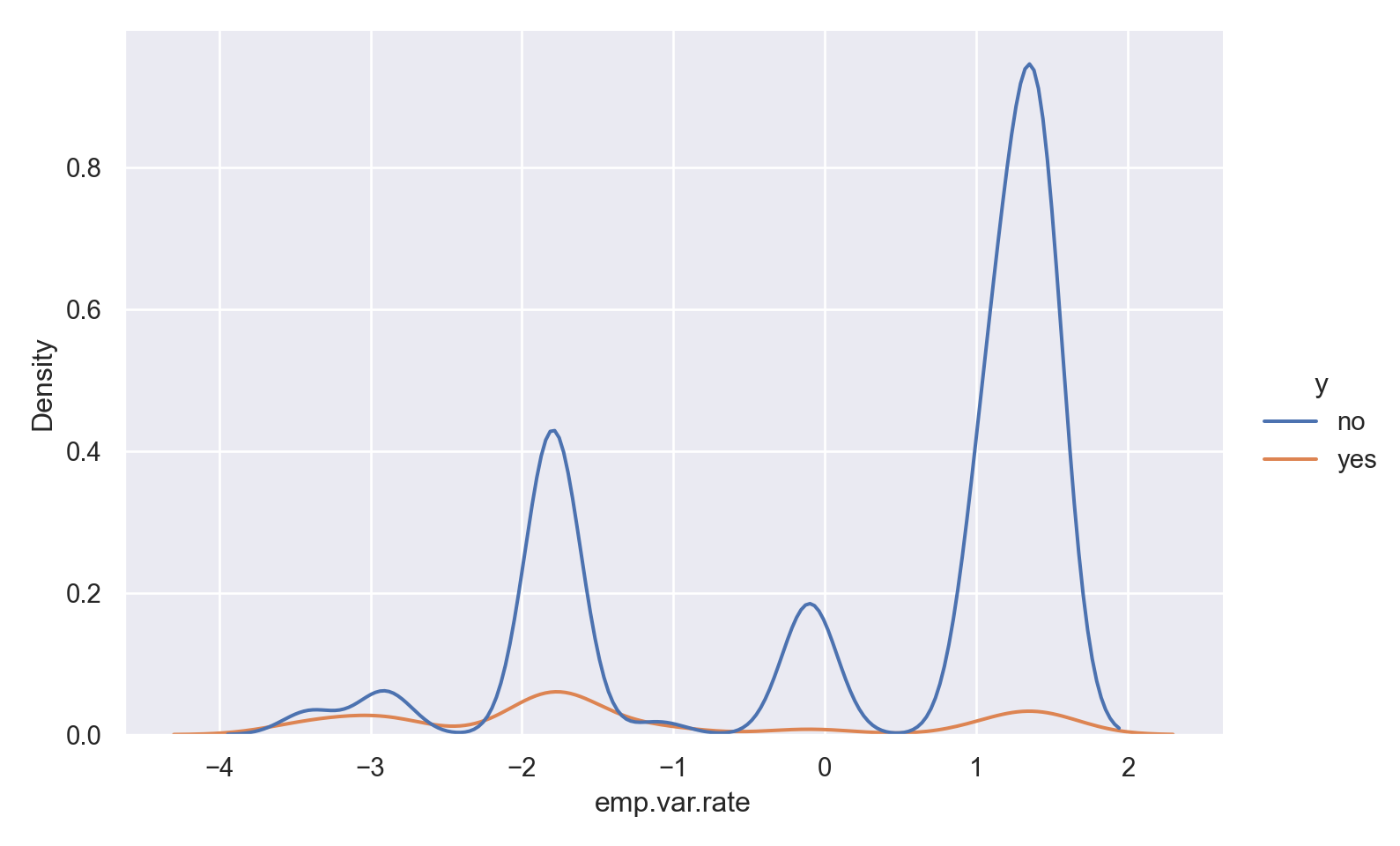

p=sns.catplot(data=data_bank_marketing, x="y", y="emp.var.rate", kind="box", height = 5, aspect = 1.5)
plt.show()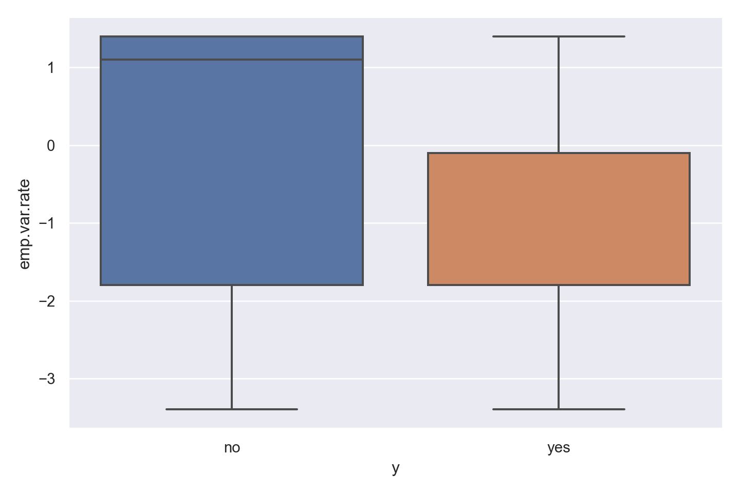

data1=rename(data, "emp.var.rate" => "emp_var_rate");
@df data1 density(:emp_var_rate, group = (:y))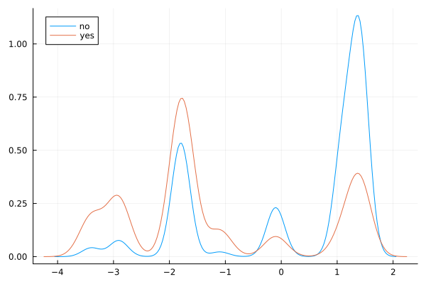

Observations

There is a striking association between employment variation rate and response - ‘yes’ outcomes show a much lower variation rate.
There is a multi-modal pattern in the data.

cons.price.idx

ggplot(data_bank_marketing) + geom_density(aes(x=cons.price.idx, color=factor(y)))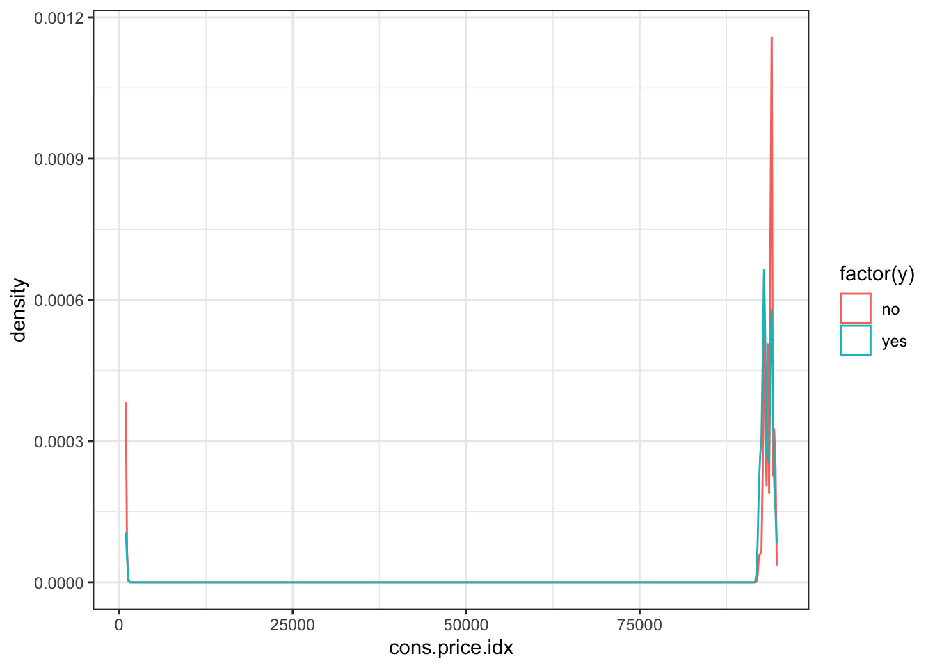

ggplot(data_bank_marketing) + geom_boxplot(aes(x=factor(y), y=cons.price.idx))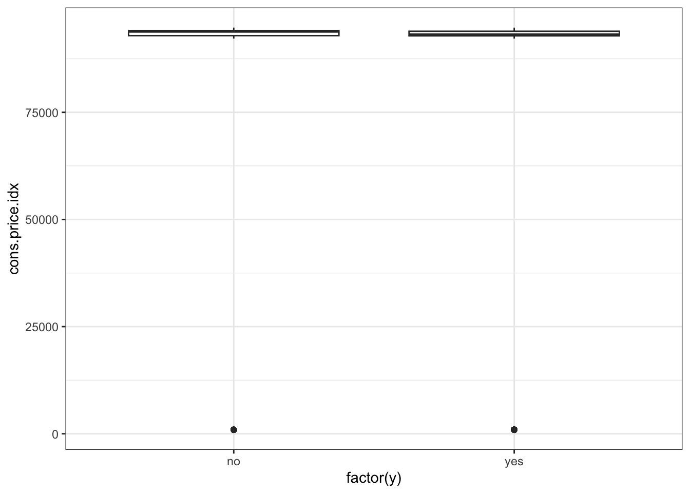

p=sns.displot(data_bank_marketing, x="cons.price.idx", hue="y", kind="kde", height = 5, aspect = 1.5)
plt.show()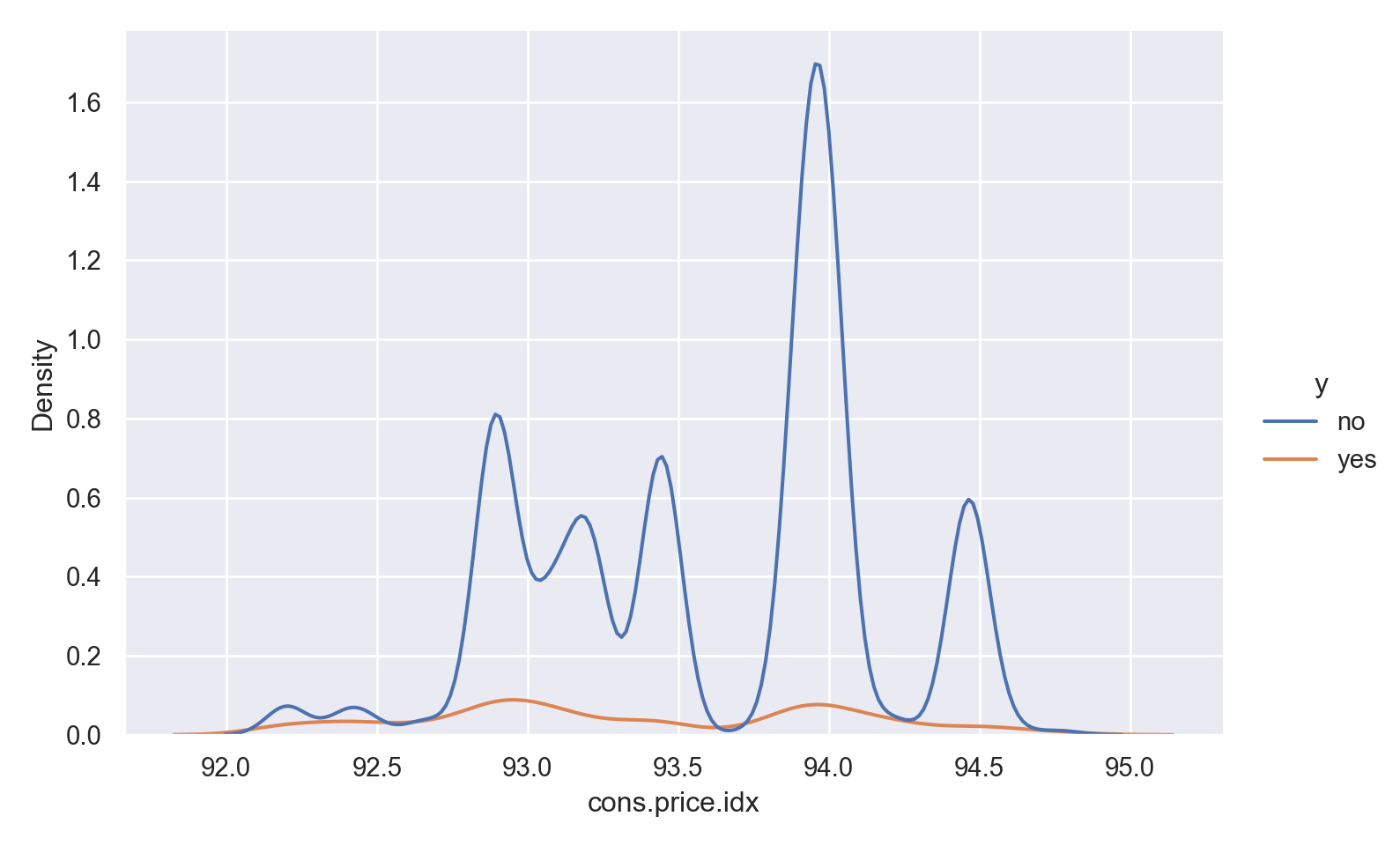

p=sns.catplot(data=data_bank_marketing, x="y", y="cons.price.idx", kind="box", height = 5, aspect = 1.5)
plt.show()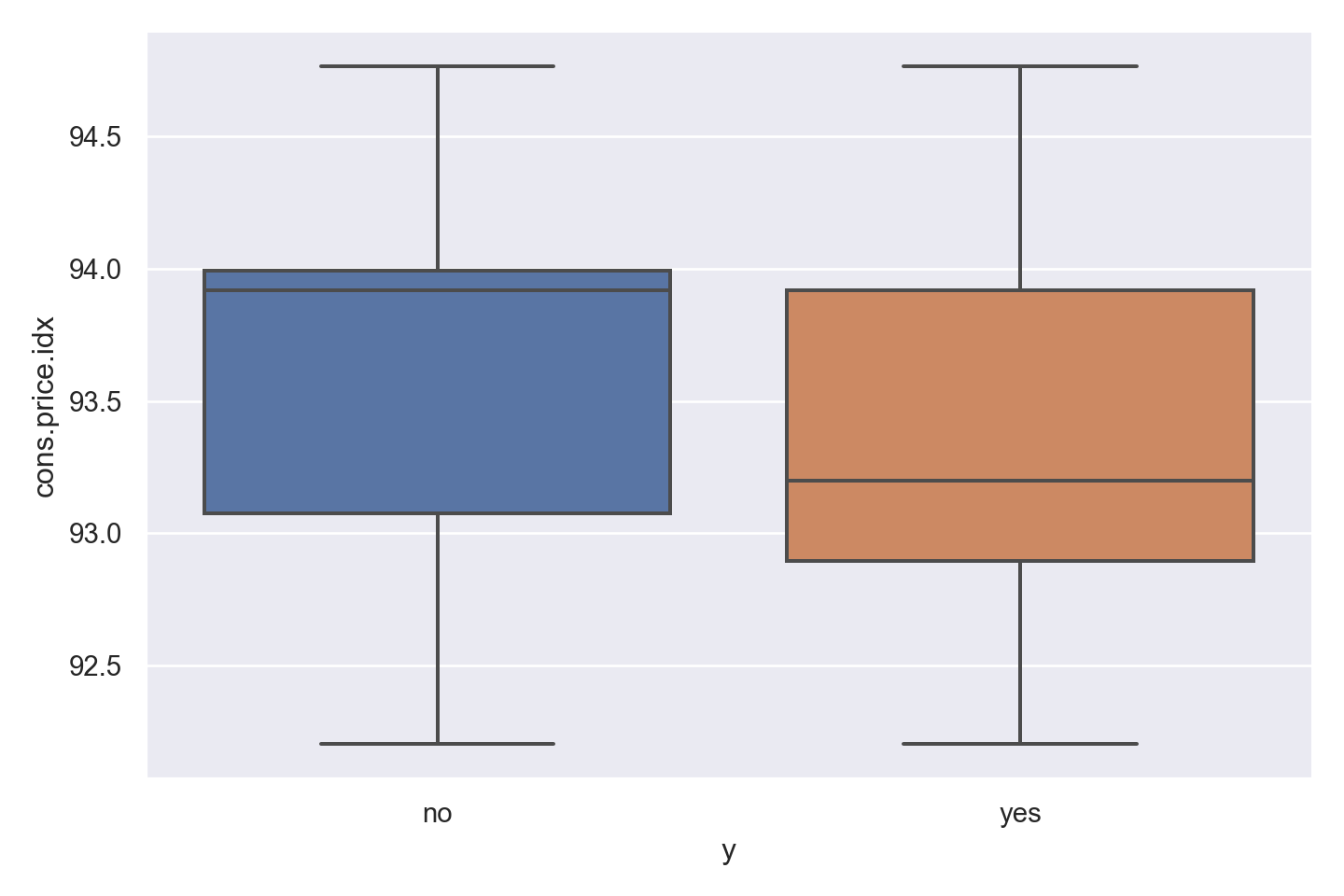

data1=rename(data, "cons.price.idx" => "cons_price_idx");
@df data1 density(:cons_price_idx, group = (:y))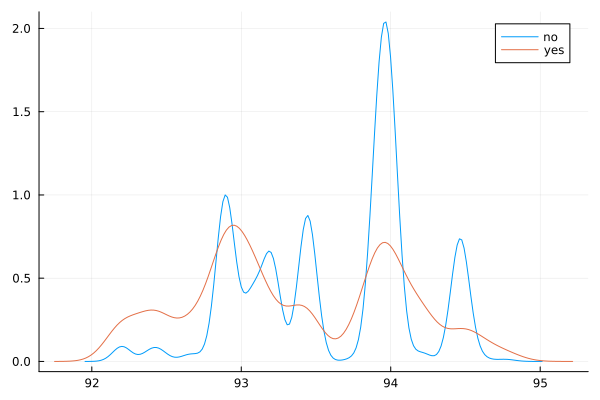

Observations

There is not much variation in the data,other than two outliers (perhaps data entry errors?)
‘yes’ outcome is associated with a slightly lower price index.

cons.conf.idx

ggplot(data_bank_marketing) + geom_density(aes(x=cons.conf.idx, color=factor(y)))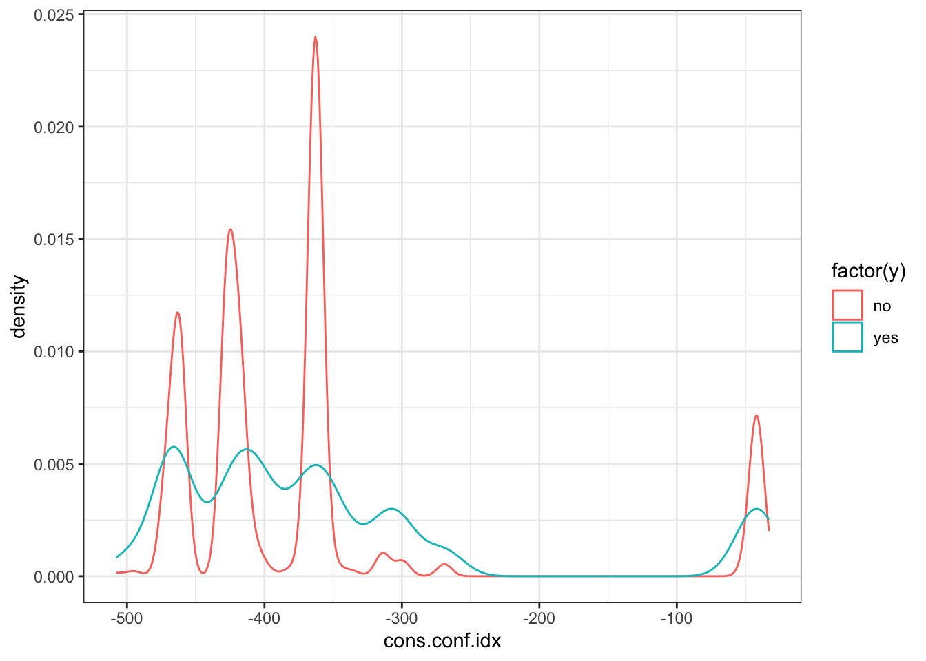

ggplot(data_bank_marketing) + geom_boxplot(aes(x=factor(y), y=cons.conf.idx))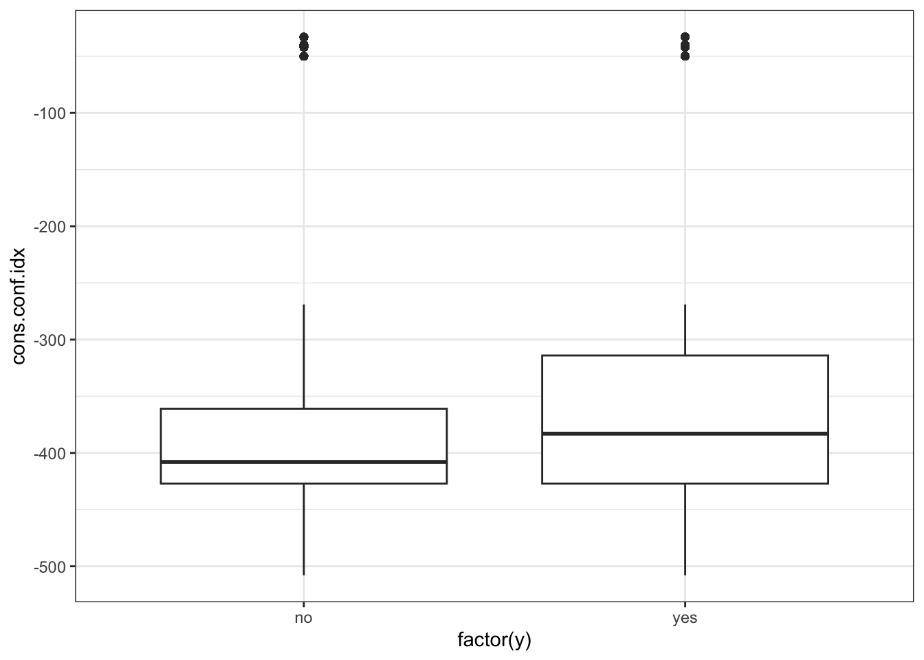

p=sns.displot(data_bank_marketing, x="cons.conf.idx", hue="y", kind="kde", height = 5, aspect = 1.5)
plt.show()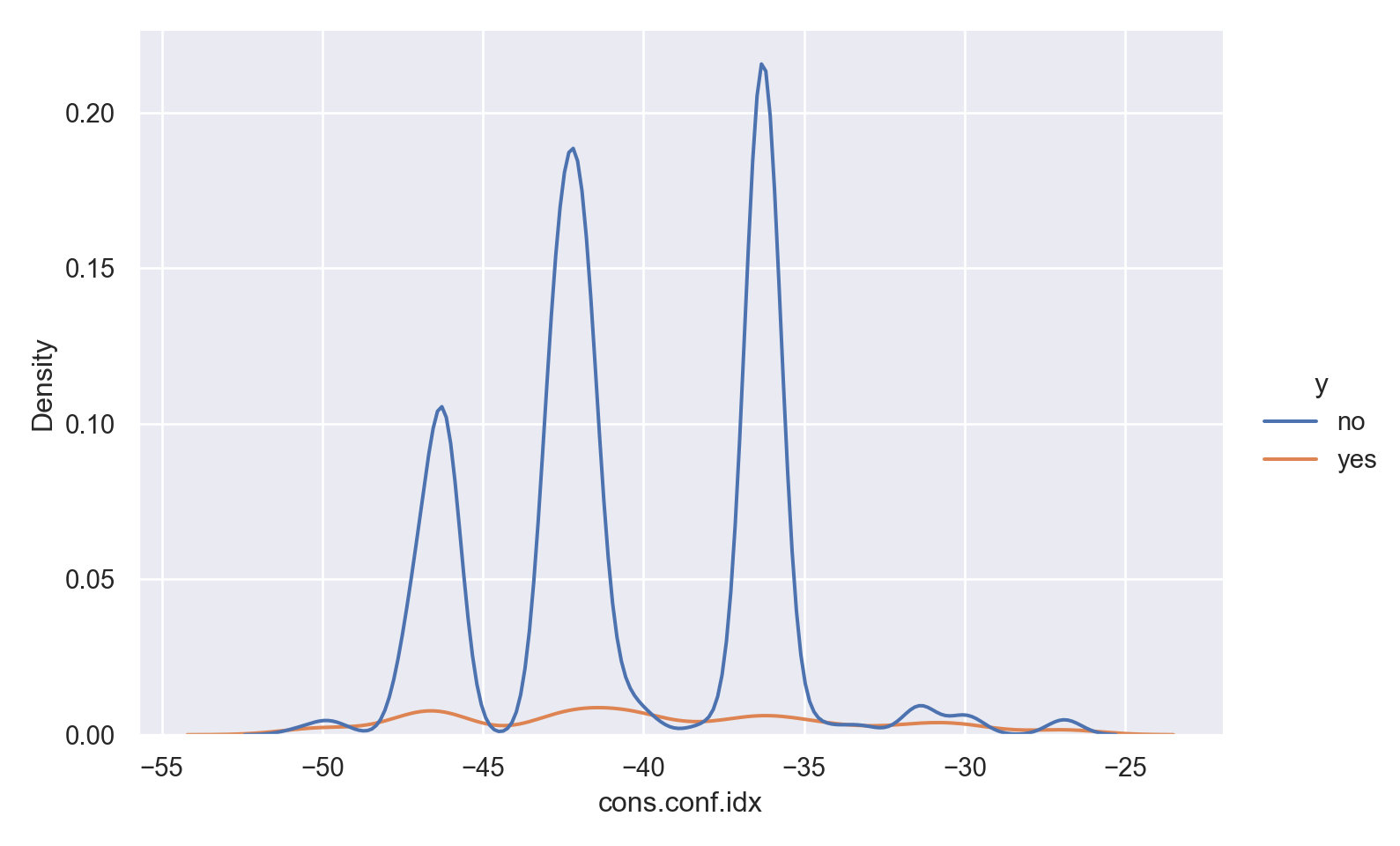

p=sns.catplot(data=data_bank_marketing, x="y", y="cons.conf.idx", kind="box", height = 5, aspect = 1.5)
plt.show()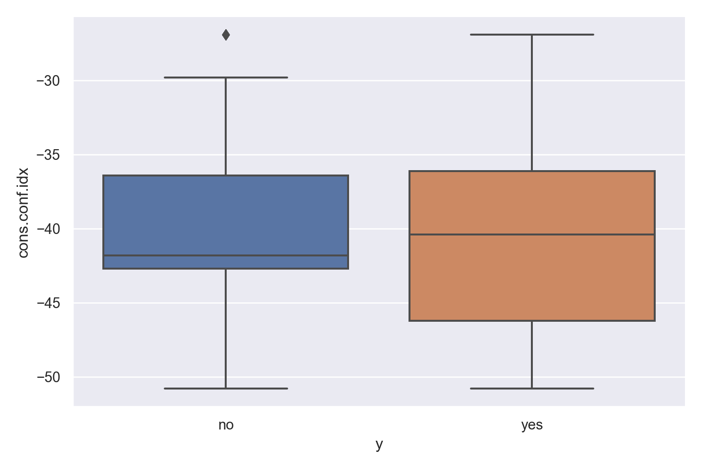

data1=rename(data, "cons.conf.idx" => "cons_conf_idx");
@df data1 density(:cons_conf_idx, group = (:y))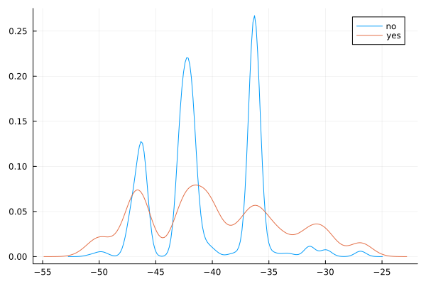

Observations

There is a strong association between confidence index and response - ‘yes’ outcomes show a higher index.
There is a multi-modal pattern in the data.

euribor3m

ggplot(data_bank_marketing) + geom_density(aes(x=euribor3m, color=factor(y)))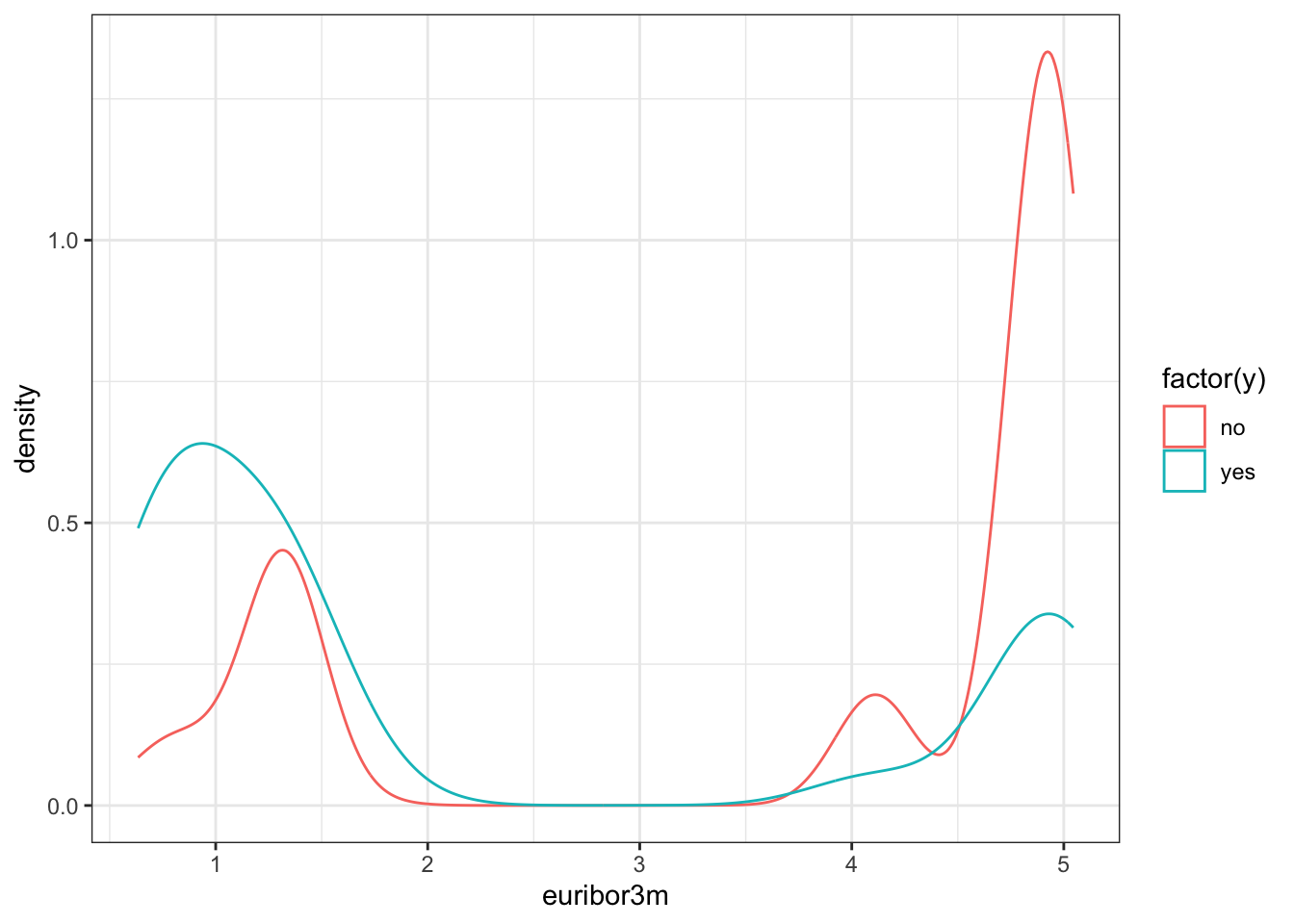

ggplot(data_bank_marketing) + geom_boxplot(aes(x=factor(y), y=euribor3m))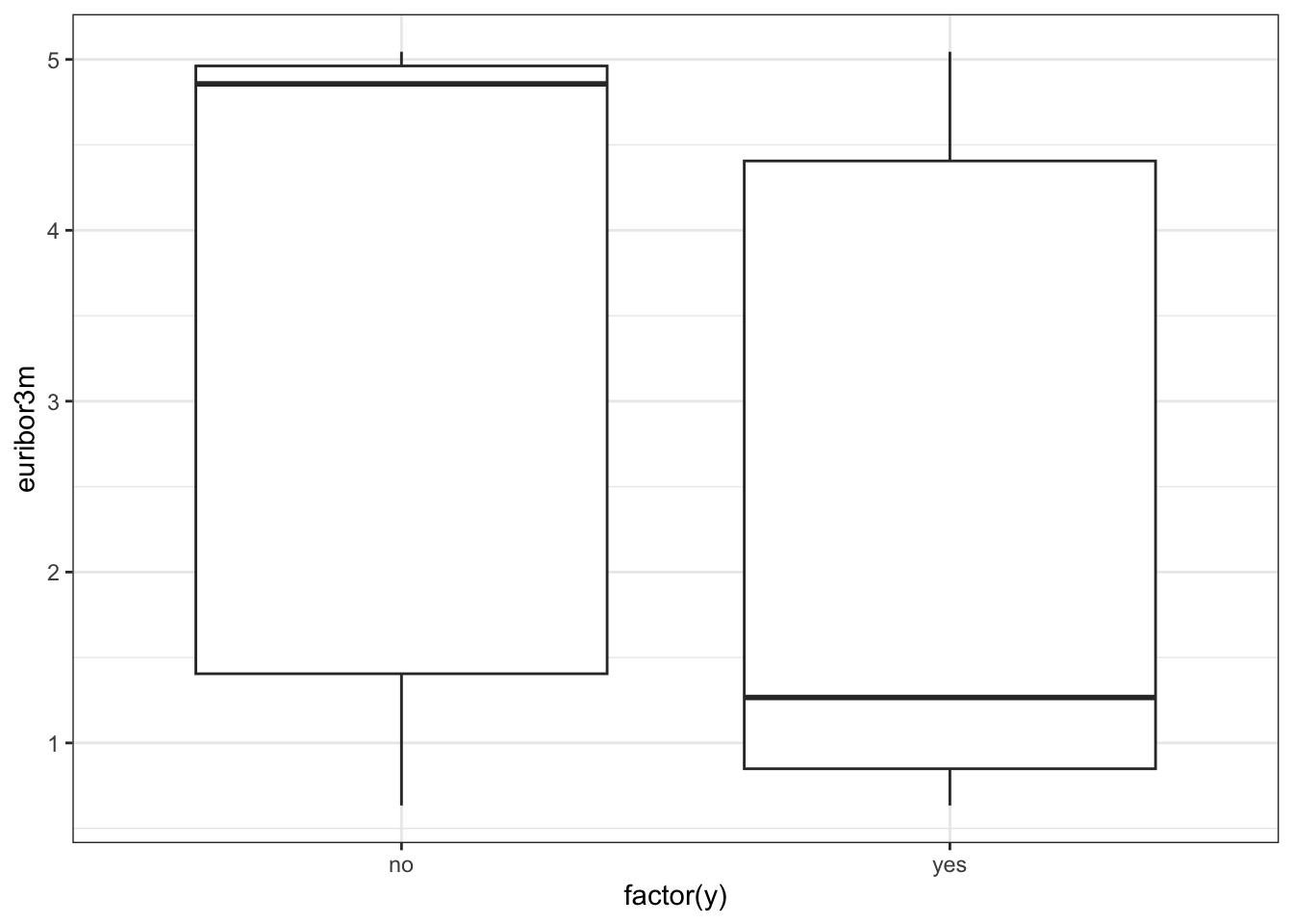

p=sns.displot(data_bank_marketing, x="euribor3m", hue="y", kind="kde", height = 5, aspect = 1.5)
plt.show()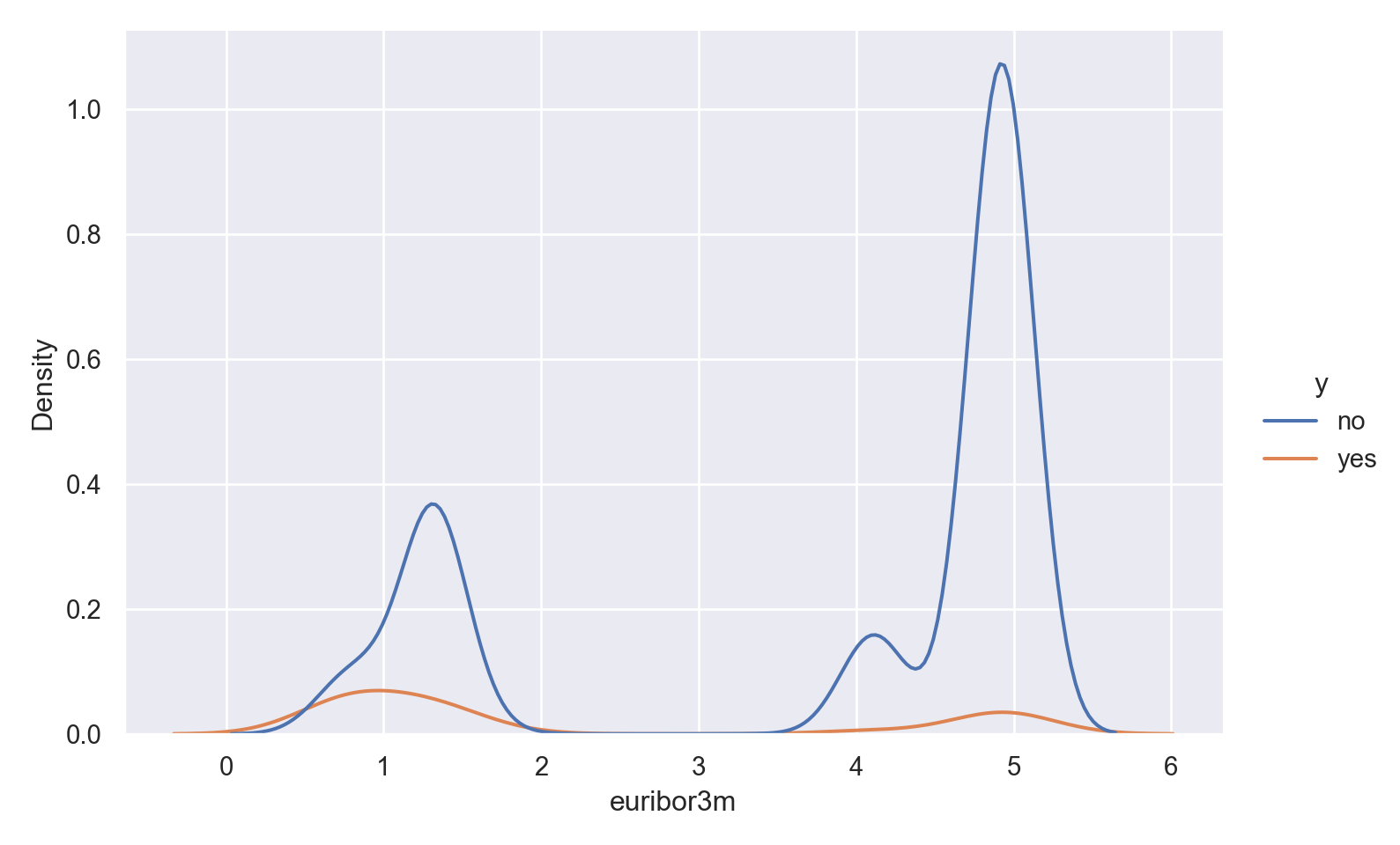

p=sns.catplot(data=data_bank_marketing, x="y", y="euribor3m", kind="box", height = 5, aspect = 1.5)
plt.show()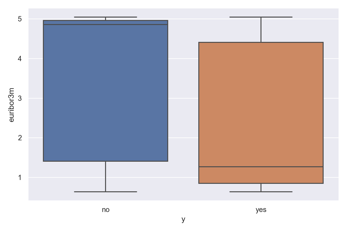

@df data density(:euribor3m, group = (:y))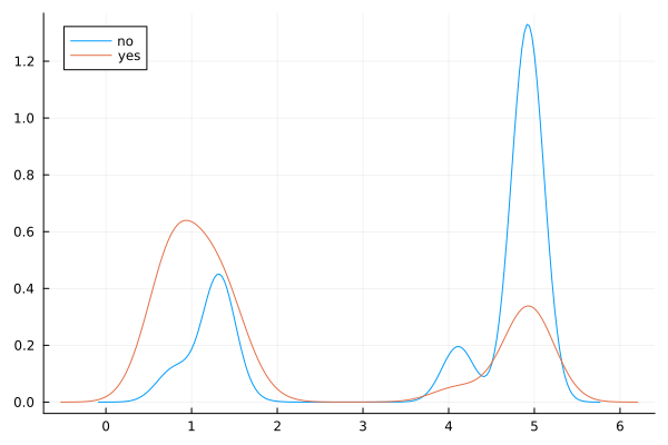

Observations

There is a striking association between employment euribor3m interest rate and response - ‘yes’ outcomes show a much lower interest rate.
There is a multi-modal pattern in the data, with more records for 1 and 5.

nr.employed

ggplot(data_bank_marketing) + geom_density(aes(x=nr.employed, color=factor(y)))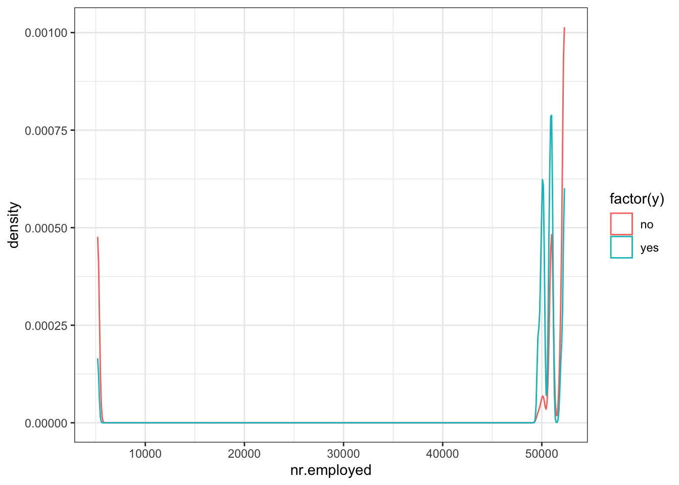

ggplot(data_bank_marketing) + geom_boxplot(aes(x=factor(y), y=nr.employed))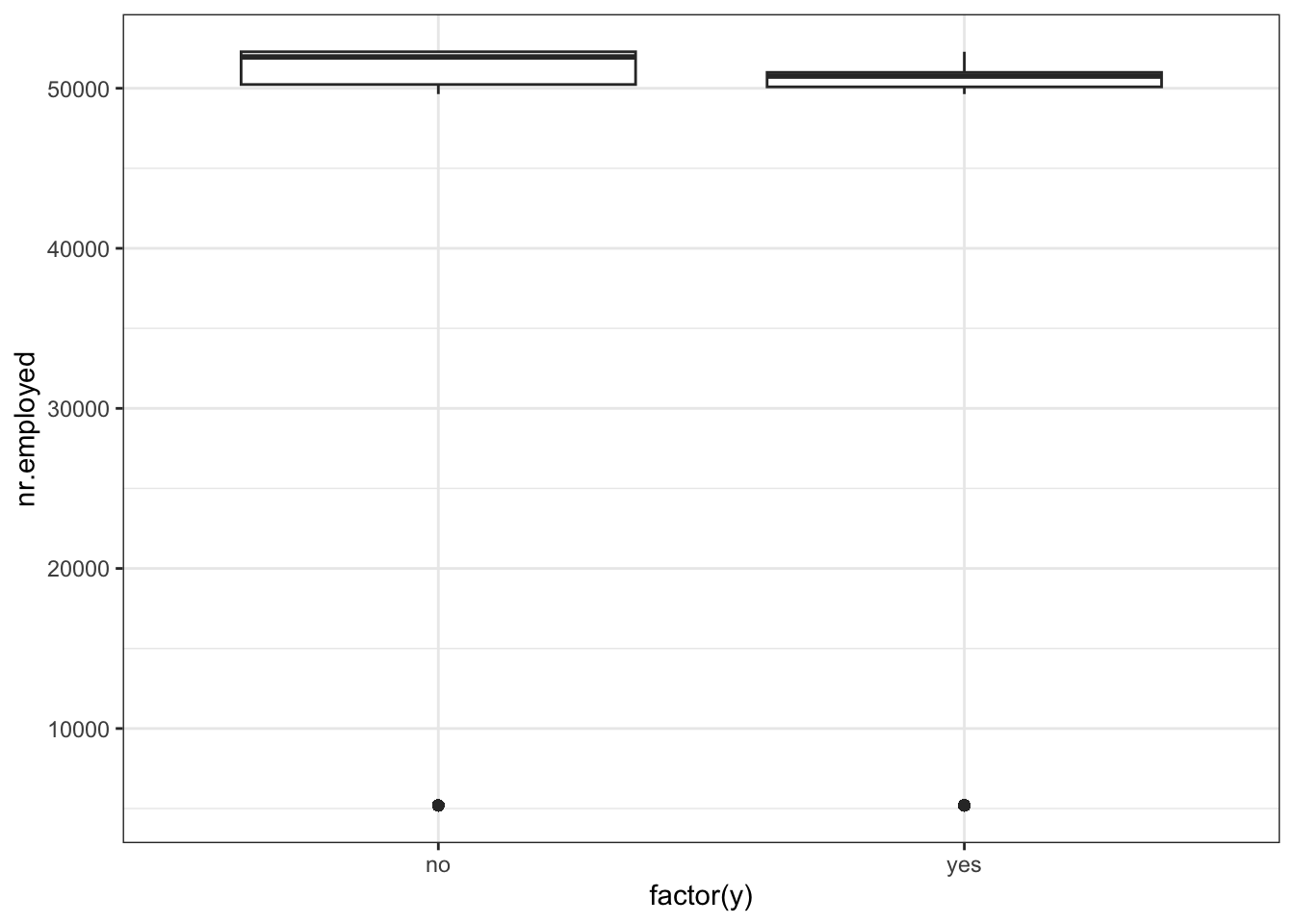

p=sns.displot(data_bank_marketing, x="nr.employed", hue="y", kind="kde", height = 5, aspect = 1.5)
plt.show()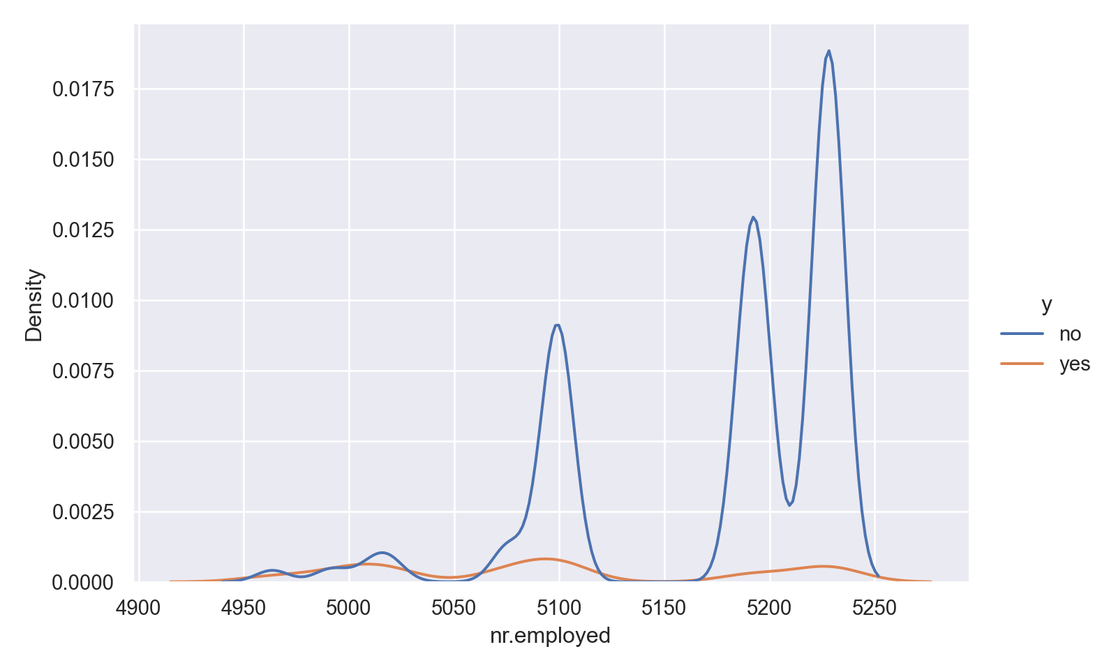

p=sns.catplot(data=data_bank_marketing, x="y", y="nr.employed", kind="box", height = 5, aspect = 1.5)
plt.show()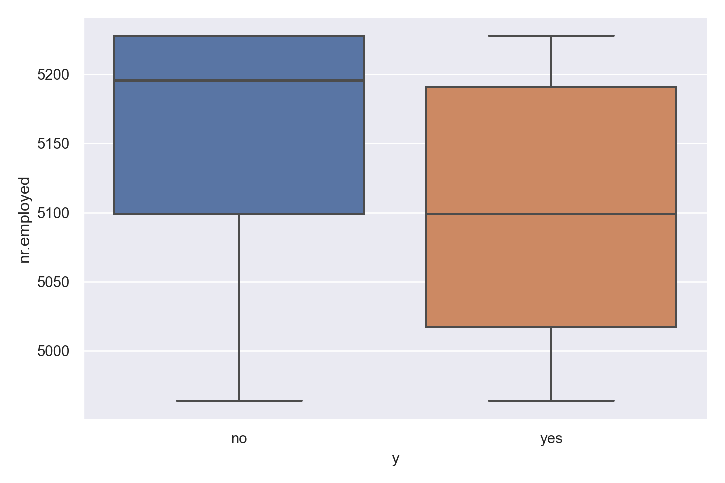

data1 = rename!(data, "nr.employed" => "nr_employed");
@df data density(:nr_employed, group = (:y))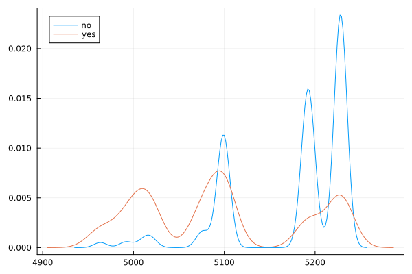

Observations

Curiously, ‘yes’ outcome is associated with a lower employment number.
There are two outliers in the data.

Categorical Attributes

job

ggplot(data_bank_marketing) + geom_bar(aes(y=factor(job), fill=factor(y)))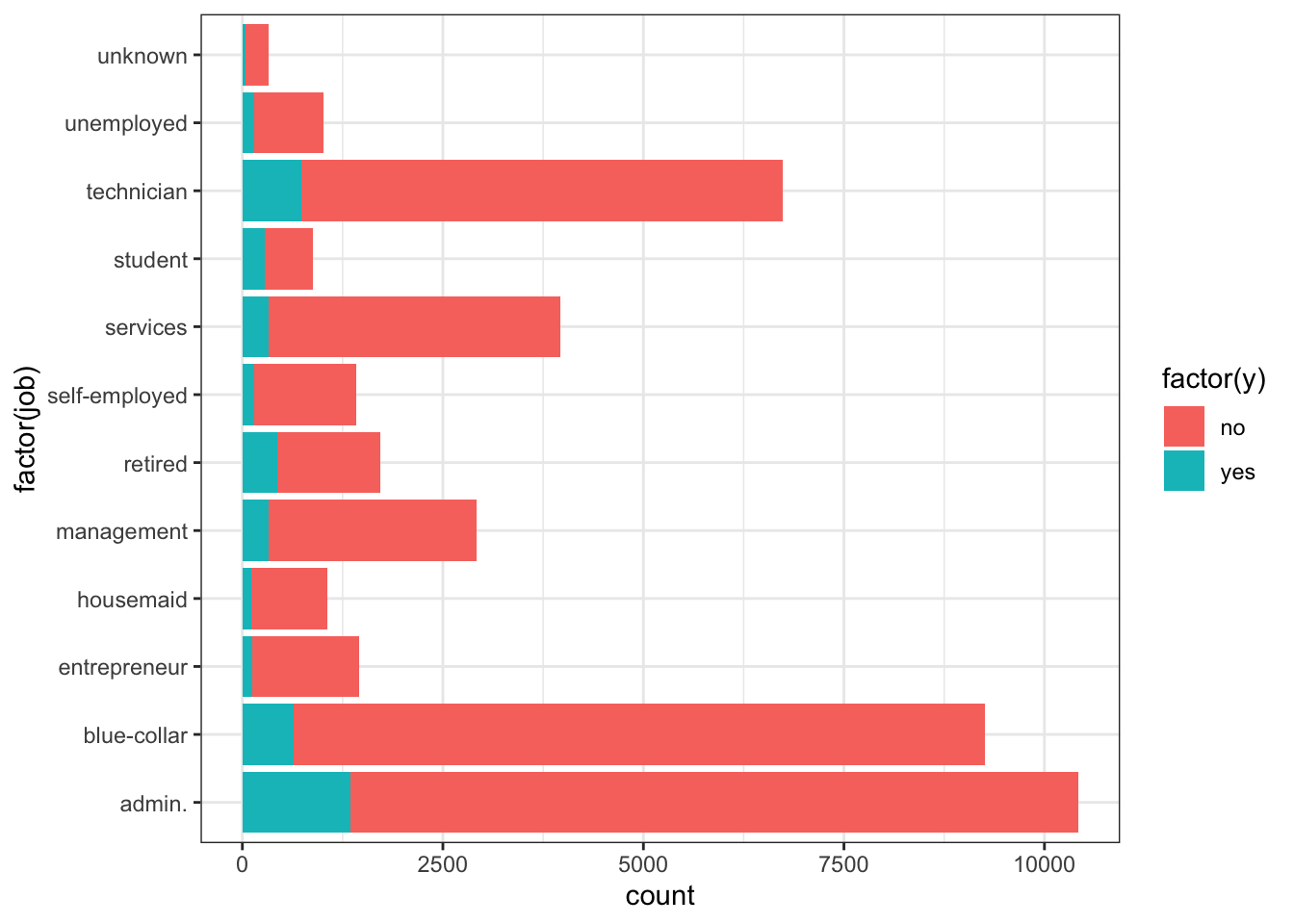

p=sns.catplot(data=data_bank_marketing, y="job", hue="y", kind="count", height = 5, aspect = 1.5)
plt.show()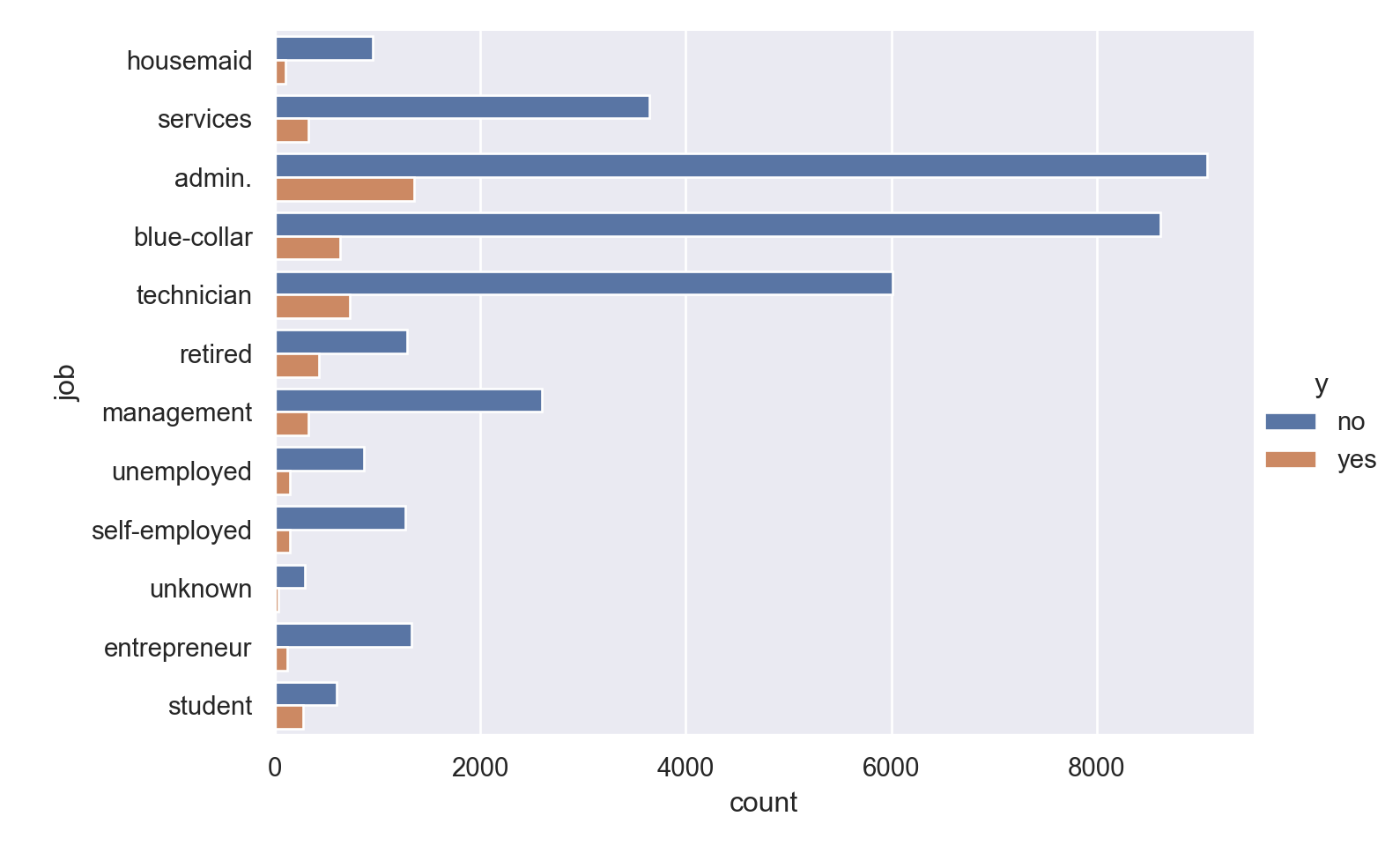

bar(countmap(data.job), xrotation=45)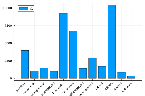

Observations

admin, blue-collar and technicians make up the majority of the people called.
There is higher percentage of yes outcome for students and retired persons, but the overall proportion of these categories is low (without being insignificant)

marital

ggplot(data_bank_marketing) + geom_bar(aes(y=factor(marital), fill=factor(y)))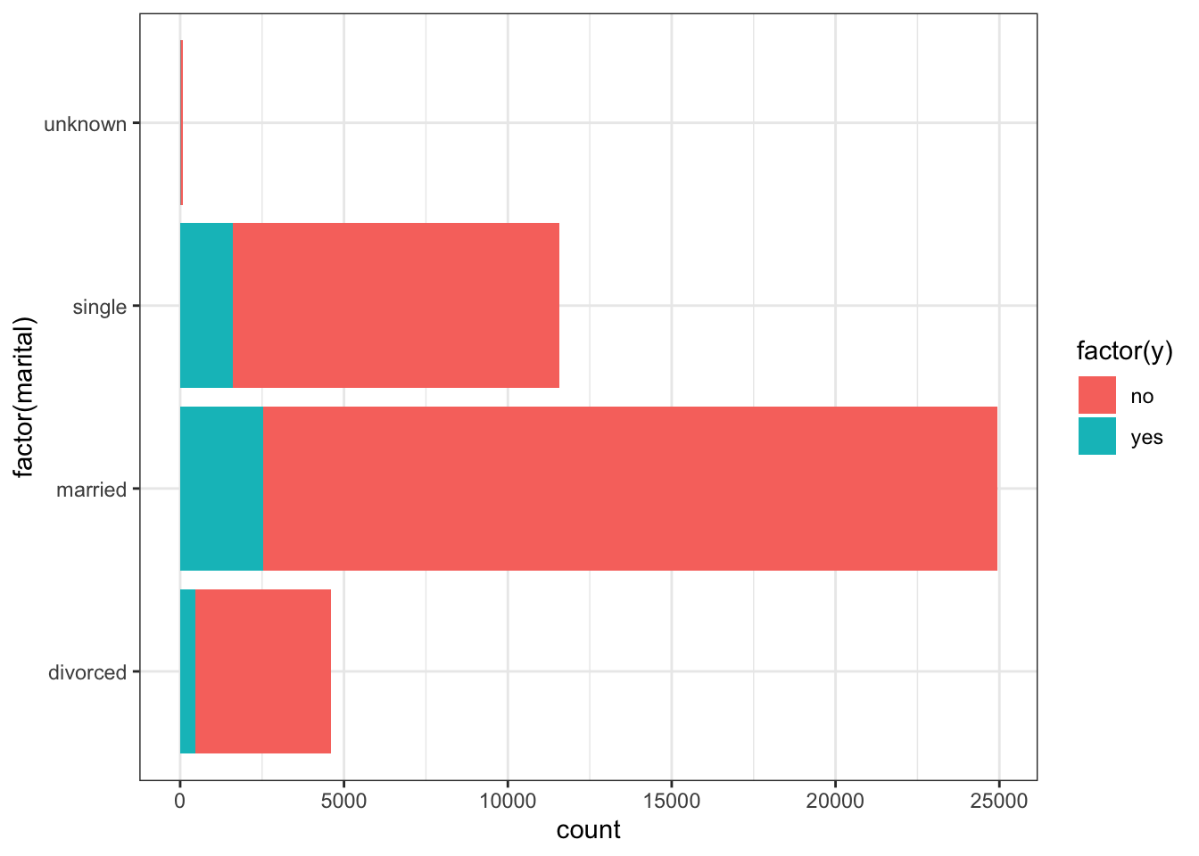

p=sns.catplot(data=data_bank_marketing, y="marital", hue="y", kind="count", height = 5, aspect = 1.5)
plt.show()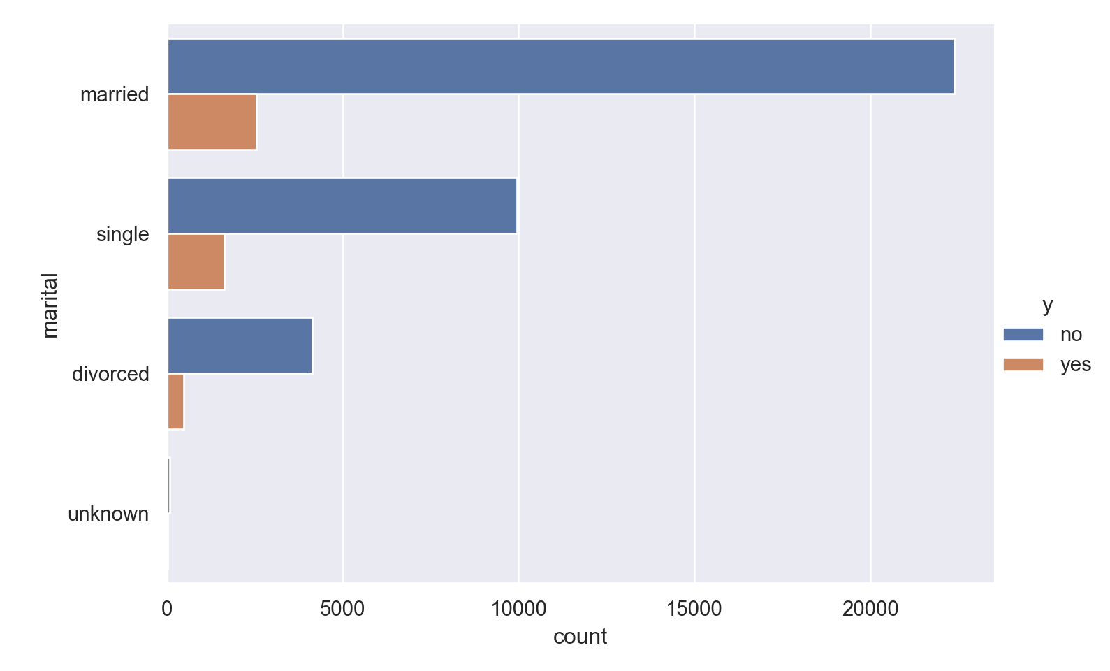

bar(countmap(data.marital))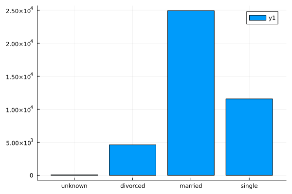

Observations

More of the people are married.
People who are single (and not divorced) have a higher proportion of ‘yes’ response.

education

ggplot(data_bank_marketing) + geom_bar(aes(y=factor(education), fill=factor(y)))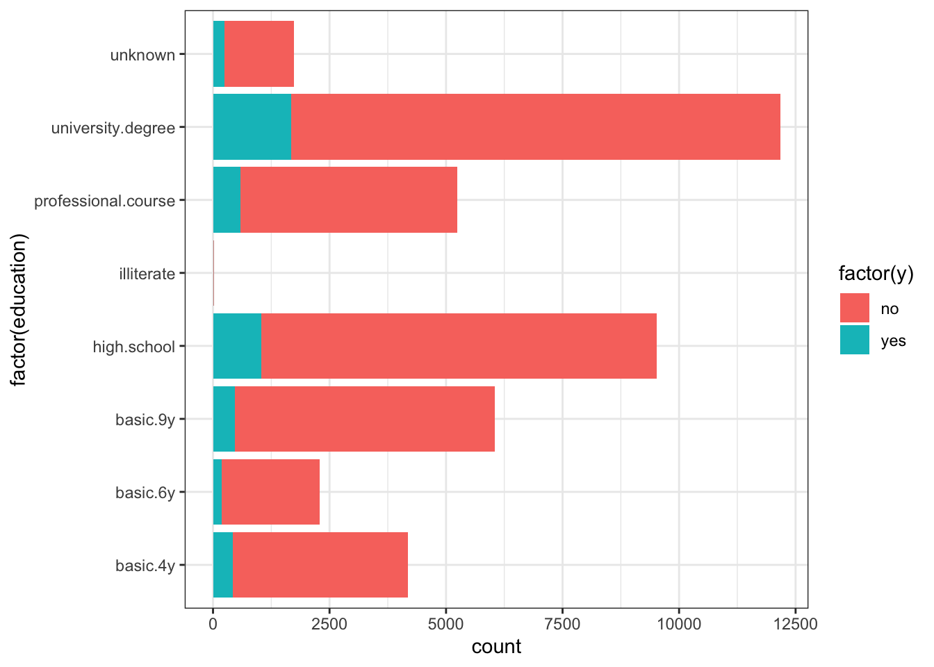

p=sns.catplot(data=data_bank_marketing, y="education", hue="y", kind="count", height = 5, aspect = 1.5)
plt.show()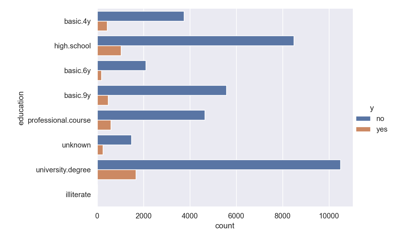

bar(countmap(data.education), xrotation=45)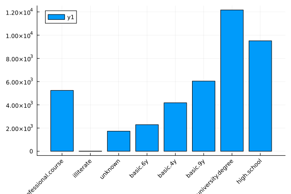

Observations

Most people called have 9 years or more education; many have a university degree.
Those with university degree show a slightly higher proportion of ‘yes’ outcome (confirmed by the numerical inspection).

default

ggplot(data_bank_marketing) + geom_bar(aes(y=factor(default), fill=factor(y)))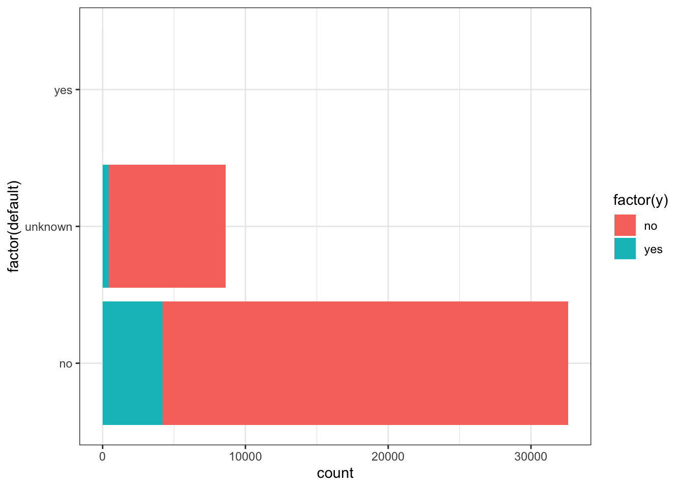

p=sns.catplot(data=data_bank_marketing, y="default", hue="y", kind="count", height = 5, aspect = 1.5)
plt.show()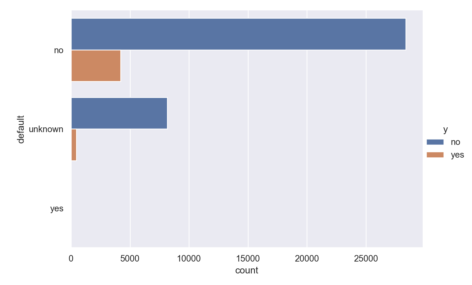

bar(countmap(data.default))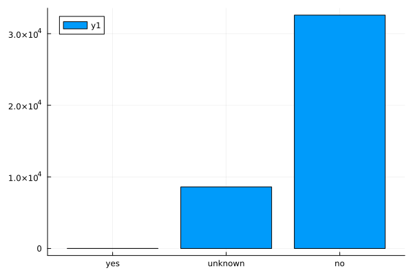

Observations

A minuscule number of the people called have a loan default.

housing

ggplot(data_bank_marketing) + geom_bar(aes(y=factor(housing), fill=factor(y)))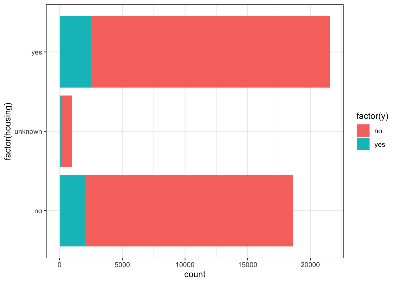

p=sns.catplot(data=data_bank_marketing, y="housing", hue="y", kind="count", height = 5, aspect = 1.5)
plt.show()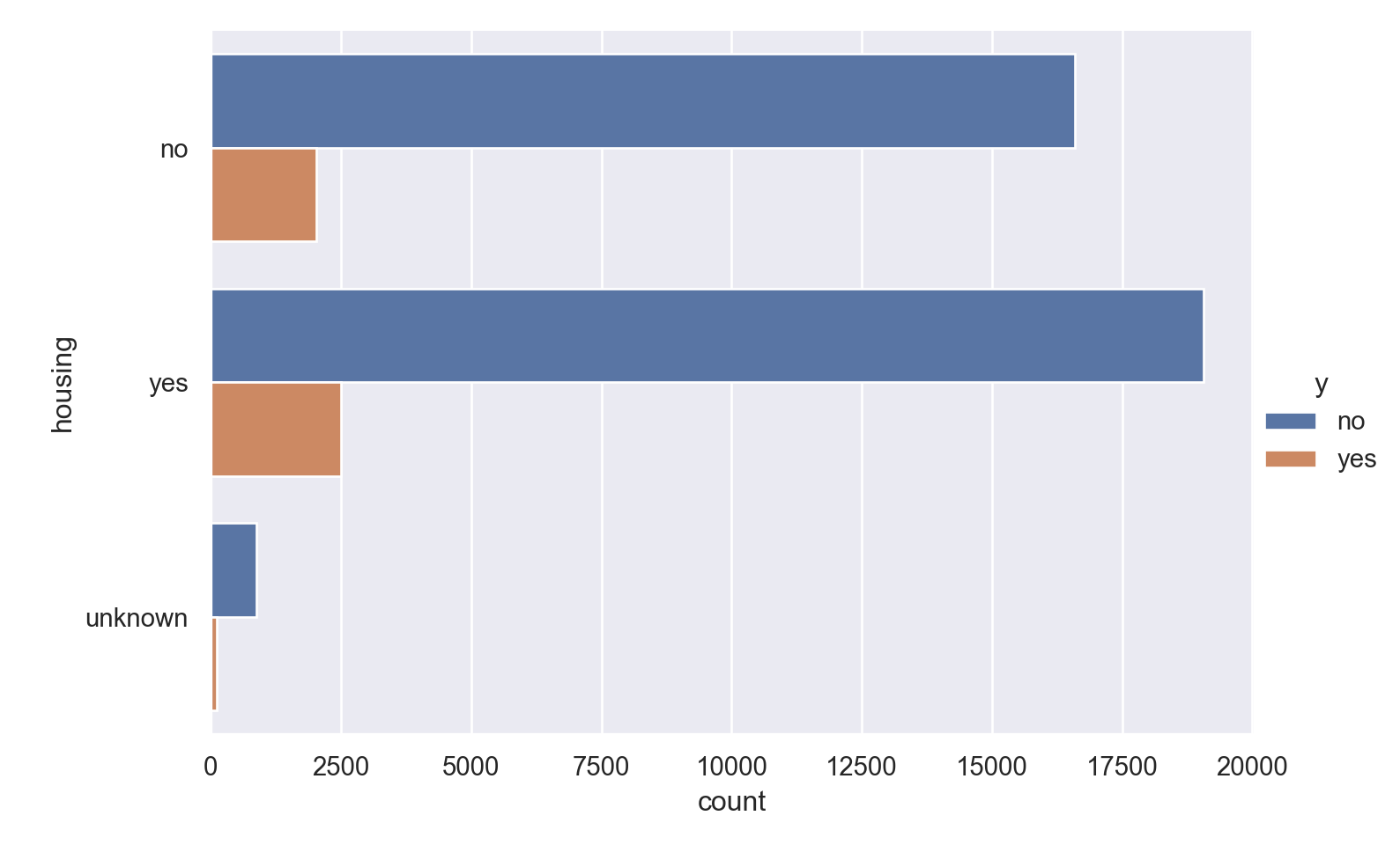

bar(countmap(data.housing))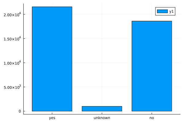

Observations

Slightly more number of people have housing.

loan

ggplot(data_bank_marketing) + geom_bar(aes(y=factor(loan), fill=factor(y)))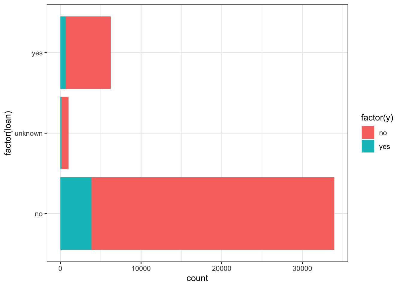

p=sns.catplot(data=data_bank_marketing, y="loan", hue="y", kind="count", height = 5, aspect = 1.5)
plt.show()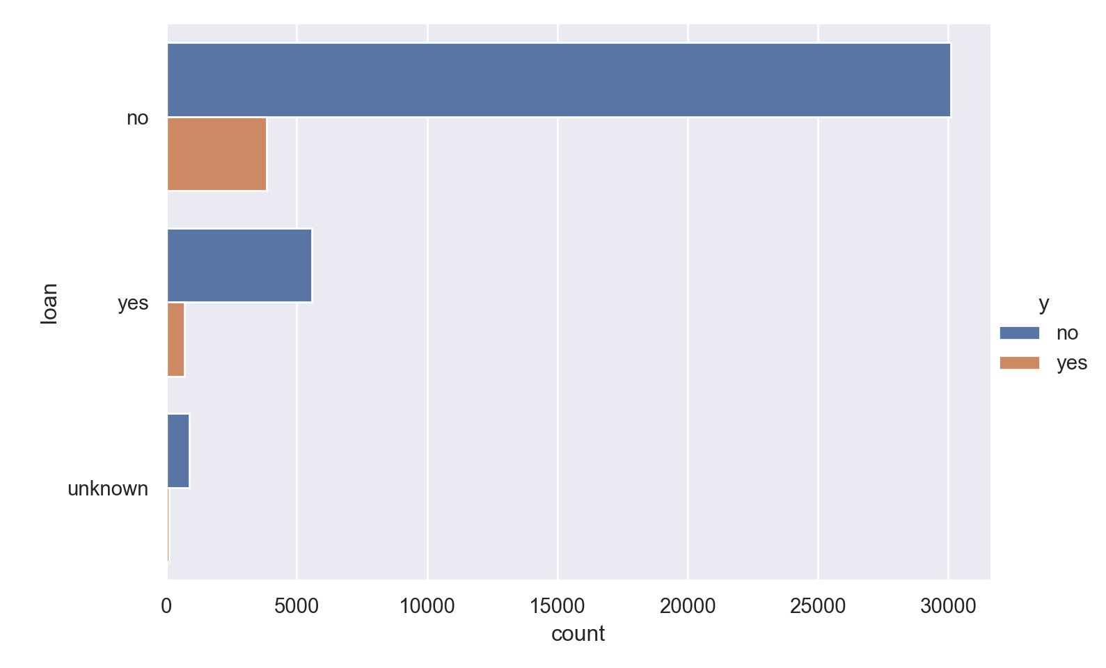

display(bar(countmap(data.loan)))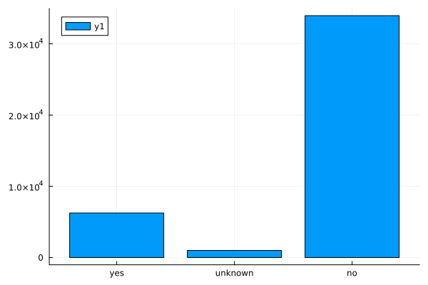

contact

ggplot(data_bank_marketing) + geom_bar(aes(y=factor(contact), fill=factor(y)))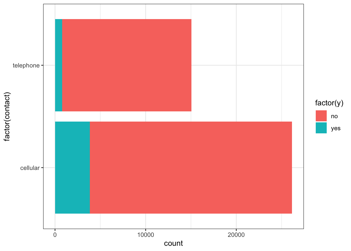

p=sns.catplot(data=data_bank_marketing, y="contact", hue="y", kind="count", height = 5, aspect = 1.5)
plt.show()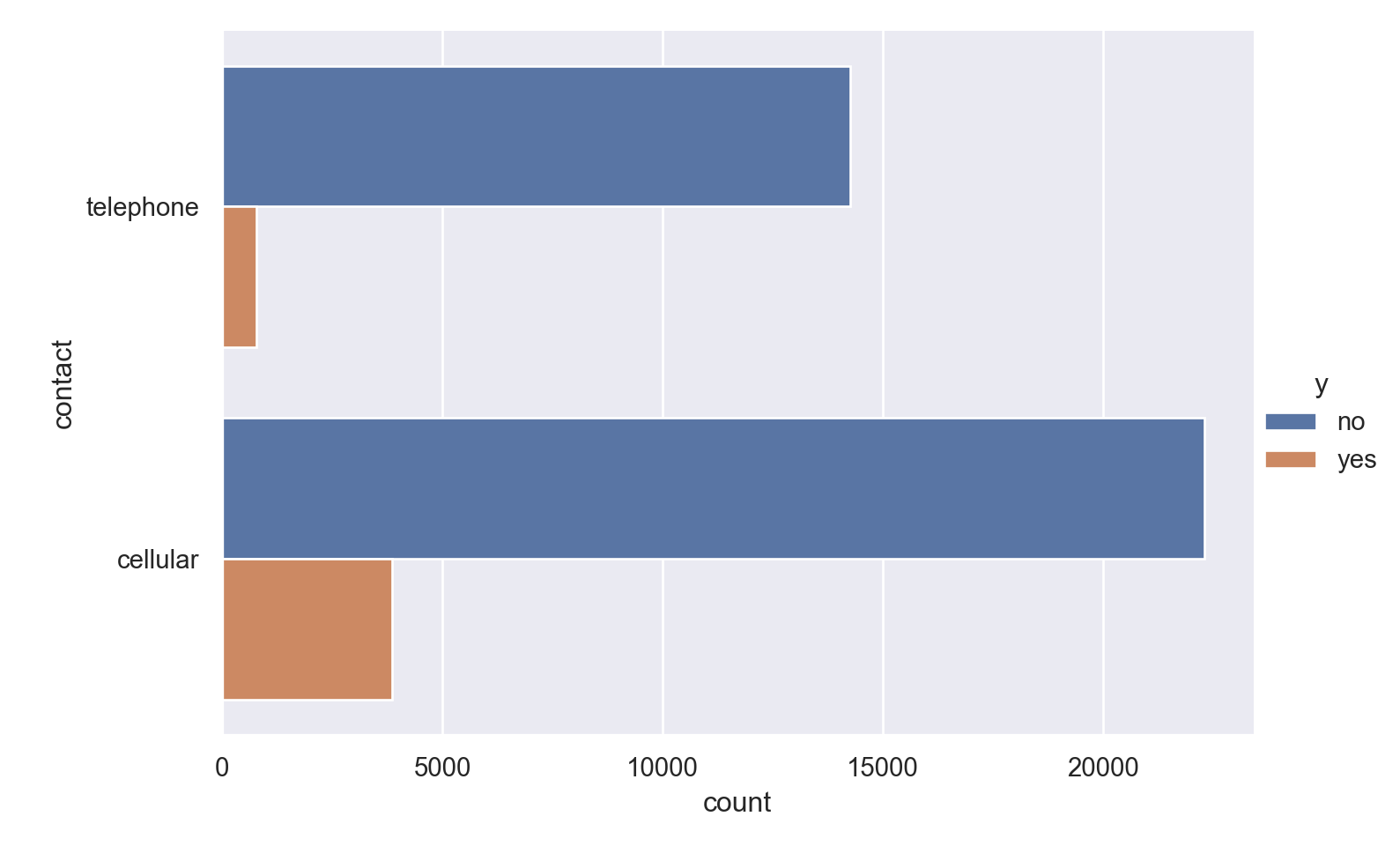

bar(countmap(data.contact))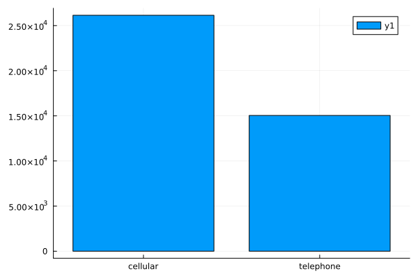

Observations

Those contacted on cellular phones have a significantly higher possibility of subscribing to the deposit.

month

ggplot(data_bank_marketing) + geom_bar(aes(y=factor(month), fill=factor(y)))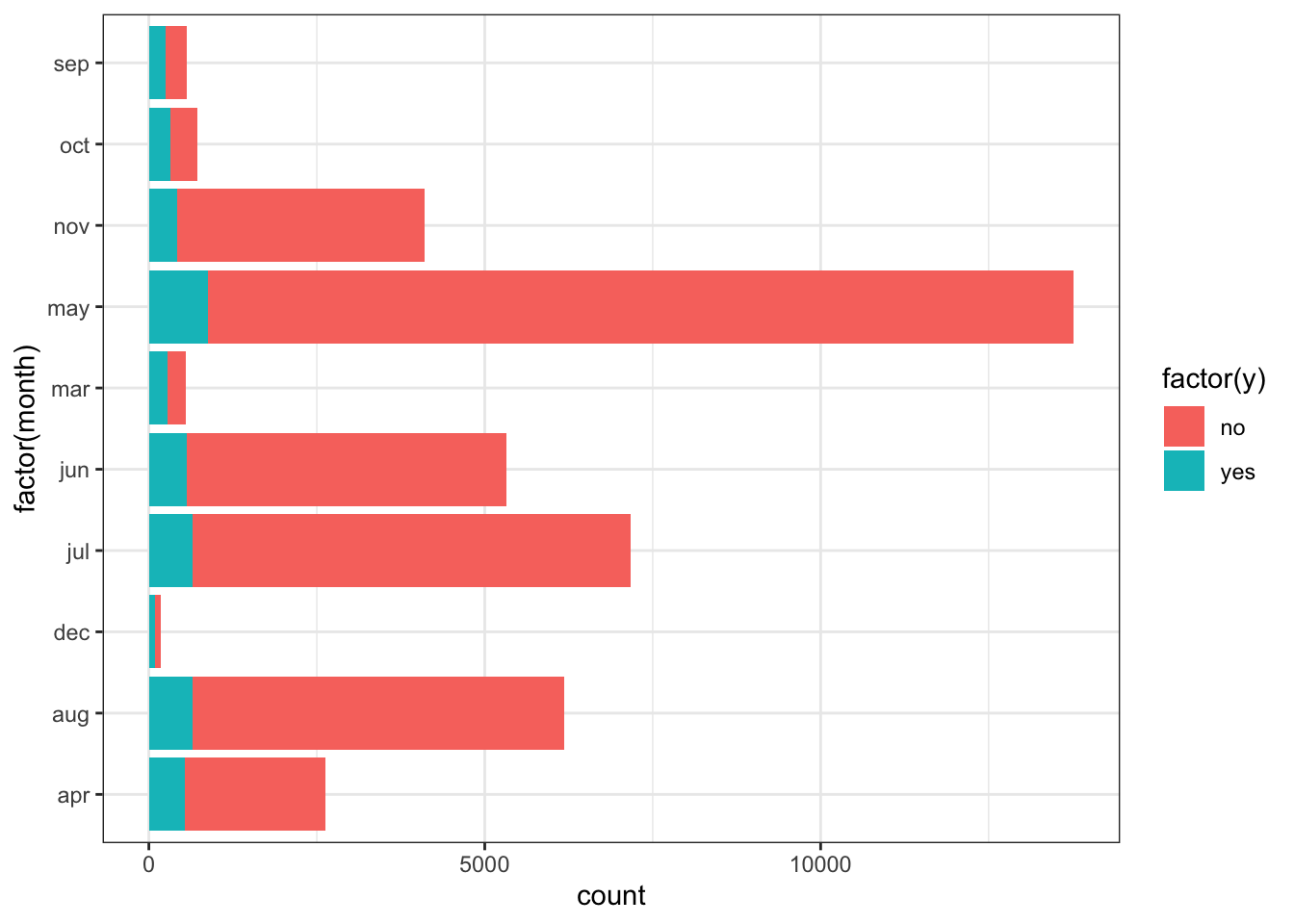

p=sns.catplot(data=data_bank_marketing, y="month", hue="y", kind="count", height = 5, aspect = 1.5)
plt.show()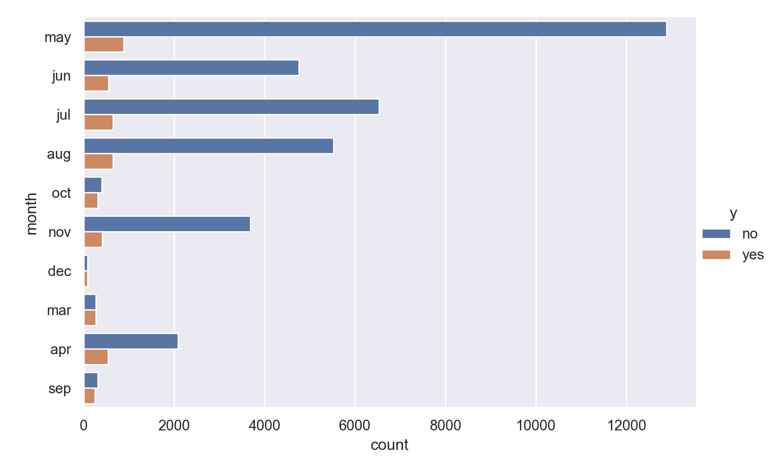

bar(countmap(data.month))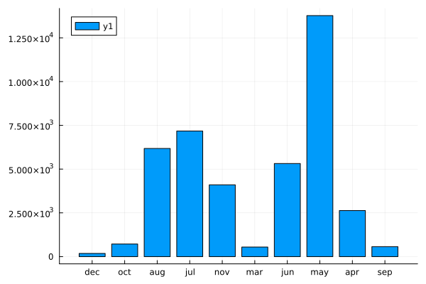

Observations

Most calls are placed in May.
The months where there were much fewer calls have a much larger chance of subscribing for the loan.

day_of_week

ggplot(data_bank_marketing) + geom_bar(aes(y=factor(day_of_week), fill=factor(y)))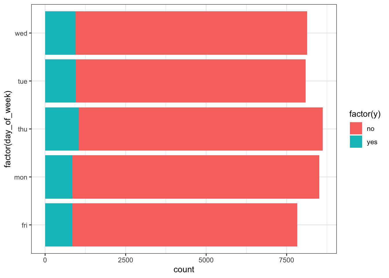

p=sns.catplot(data=data_bank_marketing, y="day_of_week", hue="y", kind="count", height = 5, aspect = 1.5)
plt.show()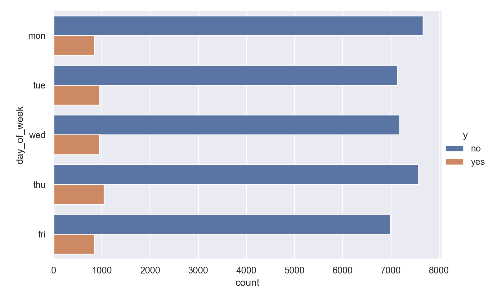

bar(countmap(data.day_of_week))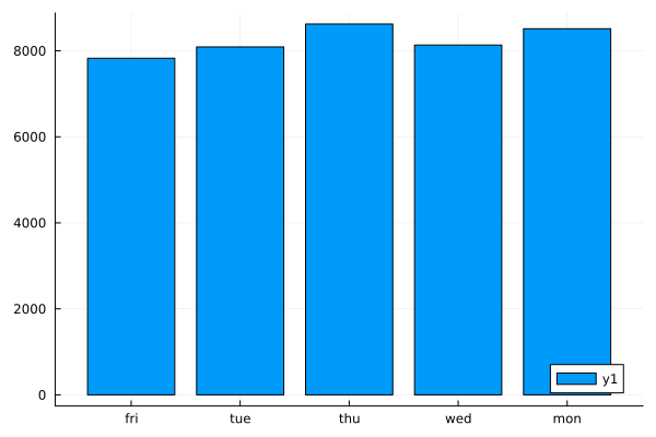

poutcome

ggplot(data_bank_marketing) + geom_bar(aes(x=factor(poutcome), fill=factor(y)))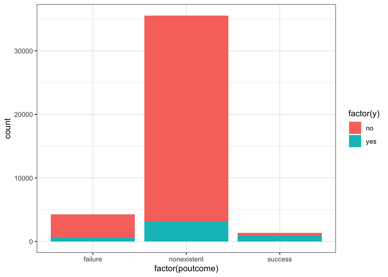

p=sns.catplot(data=data_bank_marketing, x="poutcome", hue="y", kind="count", height = 5, aspect = 1.5)
plt.show()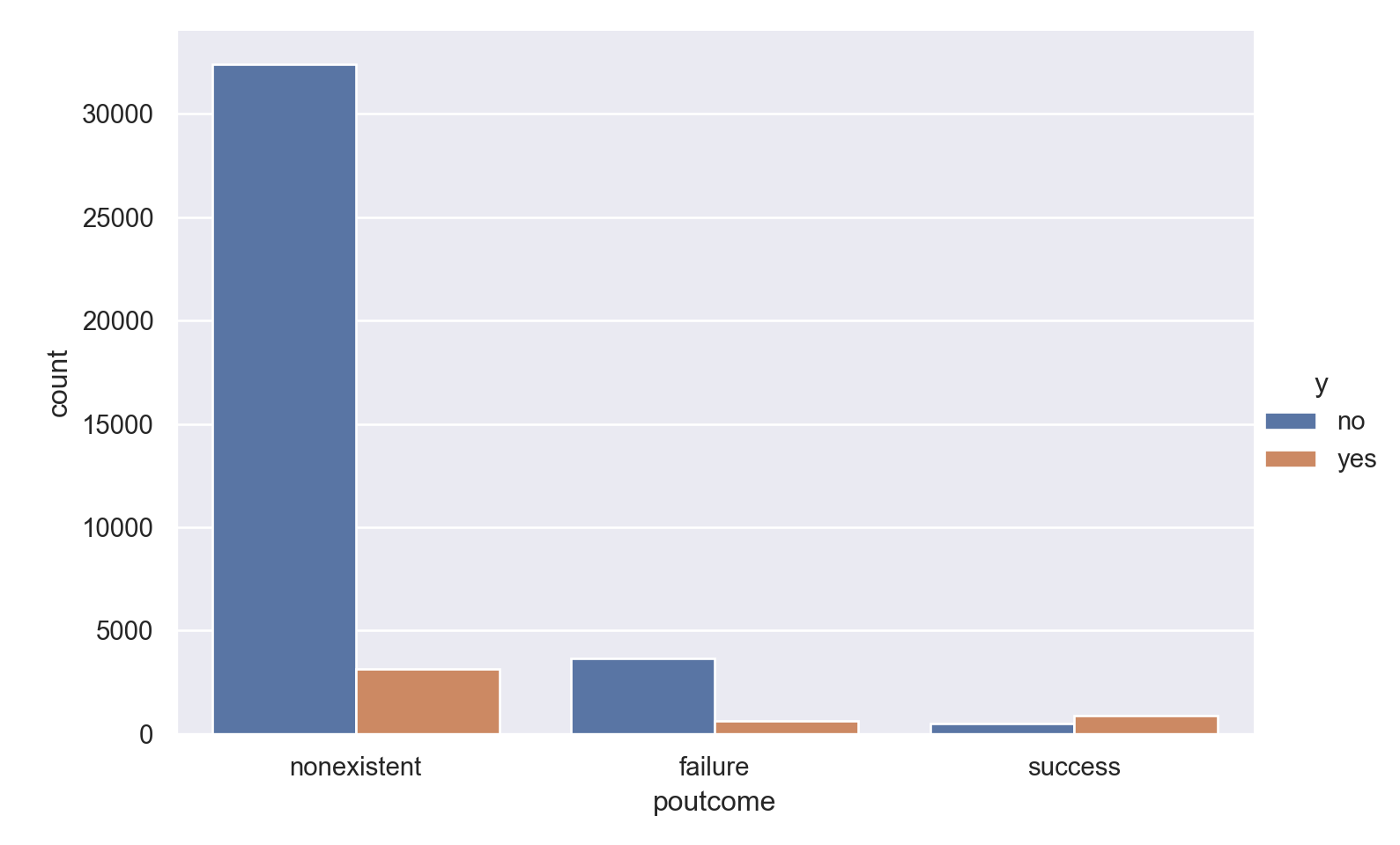

bar(countmap(data.poutcome))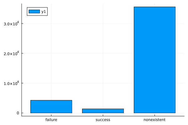

Observations

People with successful outcome in the previous campaign are much more like to have the same outcome in the current campaign.
Most people were not contacted in previous campaigns.

Training and Testing Split

set.seed(1001)
data_bank_marketing=data_bank_marketing %>% mutate(cons.conf.idx = cons.conf.idx + 509) %>% mutate(emp.var.rate = emp.var.rate + 34) %>% mutate(previous = previous + 1) %>% mutate(euribor3m = as.numeric(euribor3m))

data_bank_marketing_split = initial_split(data_bank_marketing, strata = y)

data_bank_marketing_train = training(data_bank_marketing_split)
data_bank_marketing_test  = testing(data_bank_marketing_split)

data_folds = vfold_cv(data_bank_marketing_train, strata = y)


# Global modifications applied before train\test split for effective pre-processing
data_bank_marketing["cons.conf.idx"] = data_bank_marketing["cons.conf.idx"] + 509
data_bank_marketing["emp.var.rate"] = data_bank_marketing["emp.var.rate"] + 34
data_bank_marketing["previous"] = data_bank_marketing["previous"] + 1

y = data_bank_marketing["y"]
data_bank_marketing.drop('y', axis=1, inplace=True)
data_bank_marketing.drop('duration', axis=1, inplace=True)
data_bank_marketing_train, data_bank_marketing_test, y_train, y_test = train_test_split(data_bank_marketing, y, random_state=0)

numerical_cols = data_bank_marketing_train.select_dtypes(include=['int64', 'float64']).columns
categorical_cols = data_bank_marketing_train.select_dtypes(include=['object', 'bool']).columns

log_tranform_cols = ['age', 'campaign', 'previous']
cols_index = [data_bank_marketing_train.columns.get_loc(col) for col in log_tranform_cols]

#power_transform_cols = ['cons.conf.idx', 'cons.price.idx', 'nr.employed', 'emp.var.rate', 'euribor3m']
#power_cols_index = [data_bank_marketing_train.columns.get_loc(col) for col in power_transform_cols]

#dummy_cols = ['age', 'duration', 'campaign', 'pdays', 'previous', 'emp.var.rate', 'cons.price.idx', 'cons.conf.idx', 'euribor3m', 'nr.employed']
interact_cols = ['age', 'job']
interact_cols_index = [data_bank_marketing_train.columns.get_loc(col) for col in interact_cols]
# set up the log transformer
log_transform = ColumnTransformer(
    transformers=[
        ('log', FunctionTransformer(np.log1p), cols_index),
    ],
    verbose_feature_names_out=False, # if True, "log_" will be prefixed to the column names that have been transformed
    remainder='passthrough' # this allows columns not being transformed to pass through unchanged
)

# this ensures that the transform outputs a DataFrame, so that the column names are available for the next step.
log_transform.set_output(transform='pandas')

# power = ColumnTransformer(
#     transformers=[
#         ('power', FunctionTransformer(np.square), power_cols_index),
#     ],
#     verbose_feature_names_out=False,
#     remainder='passthrough'
# )
# power.set_output(transform='pandas')

ColumnTransformer(remainder='passthrough',
                  transformers=[('log',
                                 FunctionTransformer(func=<ufunc 'log1p'>),
                                 [0, 10, 12])],
                  verbose_feature_names_out=False)

In a Jupyter environment, please rerun this cell to show the HTML representation or trust the notebook.
On GitHub, the HTML representation is unable to render, please try loading this page with nbviewer.org.

dummy = ColumnTransformer(
    transformers=[
        ('dummy', OneHotEncoder(drop='first', sparse=False), categorical_cols),
    ],
    verbose_feature_names_out=False,
    remainder='passthrough'
)

dummy.set_output(transform='pandas')

# interact = ColumnTransformer(
#     transformers=[
#         ('interact', PolynomialFeatures(interaction_only=True), interact_cols_index),
#     ],
#     verbose_feature_names_out=False,
#     remainder='passthrough'
# )
# 
# interact.set_output(transform='pandas')

ColumnTransformer(remainder='passthrough',
                  transformers=[('dummy',
                                 OneHotEncoder(drop='first', sparse=False),
                                 Index(['job', 'marital', 'education', 'default', 'housing', 'loan', 'contact', 'month', 'day_of_week', 'poutcome'], dtype='object'))],
                  verbose_feature_names_out=False)

steps=[
    ("dummy", dummy),
    ("normalize", MinMaxScaler()),
    ("zv", VarianceThreshold()),
    ]
    
pipe = Pipeline(steps)

X_trans_train = pipe.fit_transform(data_bank_marketing_train, y_train)
X_trans_test = pipe.fit_transform(data_bank_marketing_test, y_test)

# transform y
label_encoder = LabelEncoder()
y_trans_train = label_encoder.fit_transform(y_train)
y_trans_test = label_encoder.fit_transform(y_test)

coerce!(data, Textual => Multiclass);
coerce!(data, :y => OrderedFactor);

schema(data) |> DataFrames.DataFrame |> pretty_table

┌────────────────┬──────────────────┬────────────────────────────────────┐
│          names │         scitypes │                              types │
│         Symbol │         DataType │                           DataType │
├────────────────┼──────────────────┼────────────────────────────────────┤
│            age │            Count │                              Int64 │
│            job │   Multiclass{12} │ CategoricalValue{String15, UInt32} │
│        marital │    Multiclass{4} │ CategoricalValue{String15, UInt32} │
│      education │    Multiclass{8} │ CategoricalValue{String31, UInt32} │
│        default │    Multiclass{3} │  CategoricalValue{String7, UInt32} │
│        housing │    Multiclass{3} │  CategoricalValue{String7, UInt32} │
│           loan │    Multiclass{3} │  CategoricalValue{String7, UInt32} │
│        contact │    Multiclass{2} │ CategoricalValue{String15, UInt32} │
│          month │   Multiclass{10} │  CategoricalValue{String3, UInt32} │
│    day_of_week │    Multiclass{5} │  CategoricalValue{String3, UInt32} │
│       duration │            Count │                              Int64 │
│       campaign │            Count │                              Int64 │
│          pdays │            Count │                              Int64 │
│       previous │            Count │                              Int64 │
│       poutcome │    Multiclass{3} │ CategoricalValue{String15, UInt32} │
│   emp.var.rate │       Continuous │                            Float64 │
│ cons.price.idx │       Continuous │                            Float64 │
│  cons.conf.idx │       Continuous │                            Float64 │
│      euribor3m │       Continuous │                            Float64 │
│    nr_employed │       Continuous │                            Float64 │
│              y │ OrderedFactor{2} │  CategoricalValue{String3, UInt32} │
└────────────────┴──────────────────┴────────────────────────────────────┘


data_train, data_test = partition(data, 0.7, rng=42);

y_train, X_train = unpack(data_train, ==(:y), !=(:duration));
y_test, X_test = unpack(data_test, ==(:y), !=(:duration));

Transformations

Log and square transforms applied to numeric predictors.
Dummy transform needed for categorical predictors.
Interactions defined for age with job and education.

base_rec = recipe(y ~ ., data = data_bank_marketing_train) %>% step_rm(duration) #%>% step_zv(all_numeric_predictors()) %>% step_normalize(all_numeric_predictors()) %>% step_pca(all_numeric_predictors())

trfm_rec = base_rec %>% step_log(c(age, campaign, previous)) %>% step_poly(c(pdays, cons.conf.idx, cons.price.idx, nr.employed, emp.var.rate, euribor3m)) %>% step_dummy(all_nominal_predictors()) %>% step_interact(terms =~ age:starts_with("job") + age:starts_with("education"))
trfm_data = prep(trfm_rec, data_bank_marketing_train) %>% bake(new_data = NULL)


p1 = ggplot(trfm_data) + geom_density(aes(x=(campaign), color=factor(y)))
p2 = ggplot(trfm_data) + geom_density(aes(x=(age), color=factor(y)))
p3 = ggplot(trfm_data) + geom_density(aes(x=(previous), color=factor(y)))

p4 = ggplot(trfm_data) + geom_density(aes(x=(cons.conf.idx_poly_2), color=factor(y)))
p5 = ggplot(trfm_data) + geom_density(aes(x=(pdays_poly_2), color=factor(y)))

p6 = ggplot(trfm_data) + geom_density(aes(x=(cons.price.idx_poly_2), color=factor(y)))
p7 = ggplot(trfm_data) + geom_density(aes(x=(euribor3m_poly_2), color=factor(y)))
p8 = ggplot(trfm_data) + geom_density(aes(x=(nr.employed_poly_2), color=factor(y)))
p9 = ggplot(trfm_data) + geom_density(aes(x=(emp.var.rate_poly_2), color=factor(y)))

p1+p2+p3+p4 + plot_layout(ncol = 2)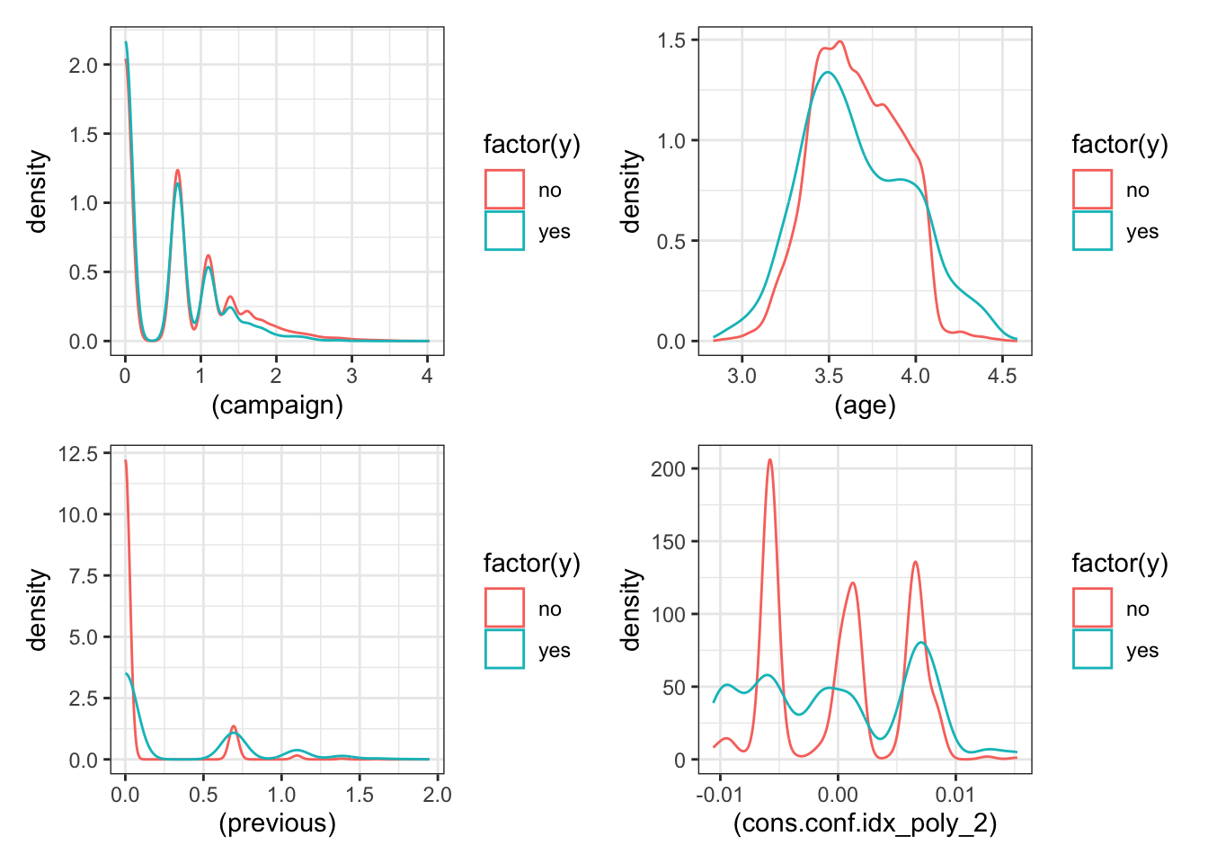

p5+p6+p7+p8+p9 + plot_layout(ncol = 2)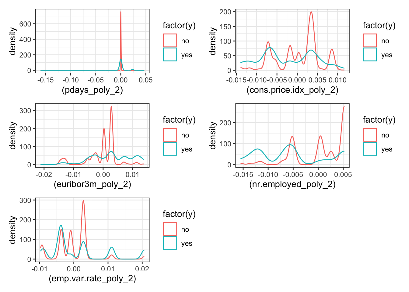


numerical_cols = data_bank_marketing_train.select_dtypes(include=['int64', 'float64']).columns
categorical_cols = data_bank_marketing_train.select_dtypes(include=['object', 'bool']).columns

log_tranform_cols = ['age', 'campaign', 'previous']
cols_index = [data_bank_marketing_train.columns.get_loc(col) for col in log_tranform_cols]

#power_transform_cols = ['cons.conf.idx', 'cons.price.idx', 'nr.employed', 'emp.var.rate', 'euribor3m']
#power_cols_index = [data_bank_marketing_train.columns.get_loc(col) for col in power_transform_cols]

#dummy_cols = ['age', 'duration', 'campaign', 'pdays', 'previous', 'emp.var.rate', 'cons.price.idx', 'cons.conf.idx', 'euribor3m', 'nr.employed']
interact_cols = ['age', 'job']
interact_cols_index = [data_bank_marketing_train.columns.get_loc(col) for col in interact_cols]
# set up the log transformer
log_transform = ColumnTransformer(
    transformers=[
        ('log', FunctionTransformer(np.log1p), cols_index),
    ],
    verbose_feature_names_out=False, # if True, "log_" will be prefixed to the column names that have been transformed
    remainder='passthrough' # this allows columns not being transformed to pass through unchanged
)

# this ensures that the transform outputs a DataFrame, so that the column names are available for the next step.
log_transform.set_output(transform='pandas')

# power = ColumnTransformer(
#     transformers=[
#         ('power', FunctionTransformer(np.square), power_cols_index),
#     ],
#     verbose_feature_names_out=False,
#     remainder='passthrough'
# )
# power.set_output(transform='pandas')

ColumnTransformer(remainder='passthrough',
                  transformers=[('log',
                                 FunctionTransformer(func=<ufunc 'log1p'>),
                                 [0, 10, 12])],
                  verbose_feature_names_out=False)

dummy = ColumnTransformer(
    transformers=[
        ('dummy', OneHotEncoder(drop='first', sparse=False), categorical_cols),
    ],
    verbose_feature_names_out=False,
    remainder='passthrough'
)

dummy.set_output(transform='pandas')

# interact = ColumnTransformer(
#     transformers=[
#         ('interact', PolynomialFeatures(interaction_only=True), interact_cols_index),
#     ],
#     verbose_feature_names_out=False,
#     remainder='passthrough'
# )
# 
# interact.set_output(transform='pandas')

ColumnTransformer(remainder='passthrough',
                  transformers=[('dummy',
                                 OneHotEncoder(drop='first', sparse=False),
                                 Index(['job', 'marital', 'education', 'default', 'housing', 'loan', 'contact', 'month', 'day_of_week', 'poutcome'], dtype='object'))],
                  verbose_feature_names_out=False)

pipe = ContinuousEncoder()

ContinuousEncoder(
  drop_last = false, 
  one_hot_ordered_factors = false)

Observations

Some of the predictors have a reduction in the skew after the transformation.

Logistic regression

glmnet_recipe <- 
  recipe(formula = y ~ ., data = data_bank_marketing_train) %>%
  step_rm(duration) %>% 
  step_log(c(age, campaign, previous)) %>% 
  #step_poly(c(pdays, cons.conf.idx, cons.price.idx, nr.employed, emp.var.rate, euribor3m)) %>% 
  ## For modeling, it is preferred to encode qualitative data as factors 
  ## (instead of character). 
  step_string2factor(one_of("job", "marital", "education", "default", "housing", 
    "loan", "contact", "month", "day_of_week", "poutcome", "y")) %>% 
  step_novel(all_nominal_predictors()) %>% 
  ## This model requires the predictors to be numeric. The most common 
  ## method to convert qualitative predictors to numeric is to create 
  ## binary indicator variables (aka dummy variables) from these 
  ## predictors. 
  step_dummy(all_nominal_predictors()) %>% 
  ## Regularization methods sum up functions of the model slope 
  ## coefficients. Because of this, the predictor variables should be on 
  ## the same scale. Before centering and scaling the numeric predictors, 
  ## any predictors with a single unique value are filtered out. 
  step_zv(all_predictors()) %>% 
  step_normalize(all_numeric_predictors()) 

glmnet_spec <- 
  multinom_reg(penalty = tune(), mixture = tune()) %>% 
  set_mode("classification") %>% 
  set_engine("glmnet") 

glmnet_workflow <- 
  workflow() %>% 
  add_recipe(glmnet_recipe) %>% 
  add_model(glmnet_spec) 

glmnet_grid <- tidyr::crossing(penalty = 10^seq(-6, -1, length.out = 20), mixture = c(0.05, 
    0.2, 0.4, 0.6, 0.8, 1)) 

# glmnet_tune <- 
  # tune_grid(glmnet_workflow, resamples = data_folds, grid = glmnet_grid, control = control_grid(save_pred = TRUE), metrics = metric_set(roc_auc)) 

final_params <-
  tibble(
    penalty = 0.0000695,
    mixture = 1
  )

final_glmnet_wflow = glmnet_workflow %>% finalize_workflow(final_params)
final_glmnet_wflow

══ Workflow ════════════════════════════════════════════════════════════════════
Preprocessor: Recipe
Model: multinom_reg()

── Preprocessor ────────────────────────────────────────────────────────────────
7 Recipe Steps

• step_rm()
• step_log()
• step_string2factor()
• step_novel()
• step_dummy()
• step_zv()
• step_normalize()

── Model ───────────────────────────────────────────────────────────────────────
Multinomial Regression Model Specification (classification)

Main Arguments:
  penalty = 6.95e-05
  mixture = 1

Computational engine: glmnet

final_glmnet_fit = final_glmnet_wflow %>% last_fit(data_bank_marketing_split)

final_glmnet_fit %>% collect_metrics()

# A tibble: 2 × 4
  .metric  .estimator .estimate .config             
  <chr>    <chr>          <dbl> <chr>               
1 accuracy binary         0.901 Preprocessor1_Model1
2 roc_auc  binary         0.793 Preprocessor1_Model1

final_glmnet_fit %>% collect_predictions()

# A tibble: 10,297 × 7
   id               .pred_no .pred_yes  .row .pred_class y     .config          
   <chr>               <dbl>     <dbl> <int> <fct>       <fct> <chr>            
 1 train/test split    0.970    0.0299     7 no          no    Preprocessor1_Mo…
 2 train/test split    0.977    0.0225    18 no          no    Preprocessor1_Mo…
 3 train/test split    0.968    0.0321    21 no          no    Preprocessor1_Mo…
 4 train/test split    0.980    0.0201    22 no          no    Preprocessor1_Mo…
 5 train/test split    0.970    0.0296    24 no          no    Preprocessor1_Mo…
 6 train/test split    0.985    0.0155    30 no          no    Preprocessor1_Mo…
 7 train/test split    0.977    0.0230    34 no          no    Preprocessor1_Mo…
 8 train/test split    0.975    0.0255    35 no          no    Preprocessor1_Mo…
 9 train/test split    0.969    0.0313    43 no          no    Preprocessor1_Mo…
10 train/test split    0.973    0.0265    52 no          no    Preprocessor1_Mo…
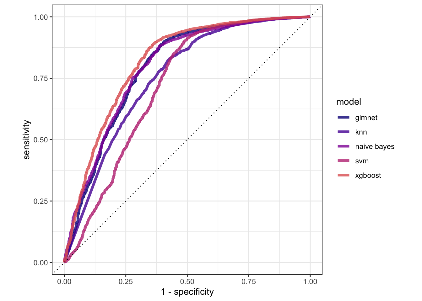
# … with 10,287 more rows

final_glmnet_fit %>% collect_predictions() %>% roc_curve(y, .pred_no) %>% autoplot()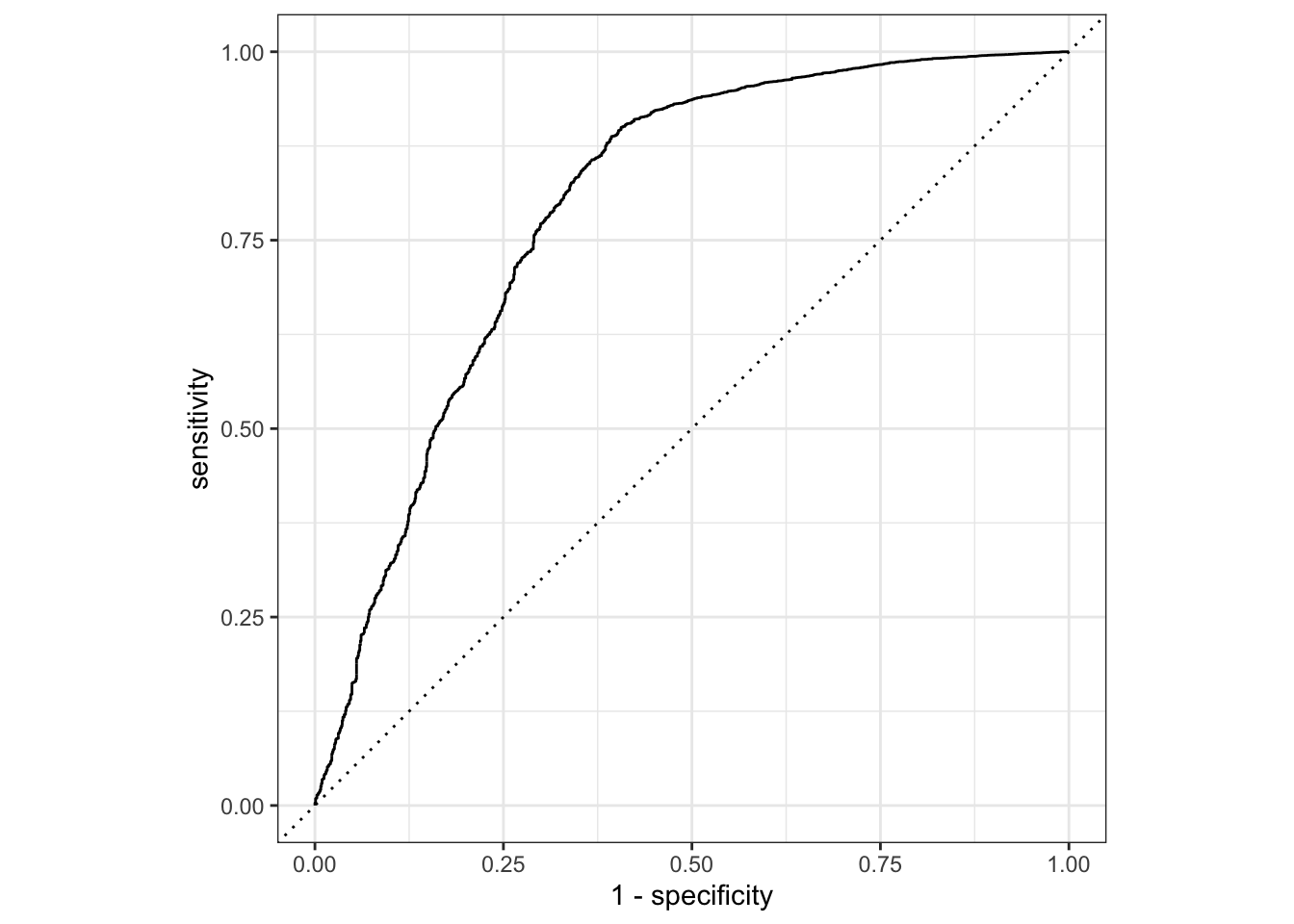

glmnet_auc = final_glmnet_fit %>% collect_predictions() %>% roc_curve(y, .pred_no) %>% mutate(model = "glmnet")


def roc_plot(X_test,Y_test, fitted_model, pos_label='yes'):
  # calculate the fpr and tpr for all thresholds of the classification
  probs = fitted_model.predict_proba(X_test)
  probs_no = probs[:,1]
  fpr, tpr, threshold = metrics.roc_curve(Y_test, probs_no, pos_label = pos_label)
  roc_auc = metrics.auc(fpr, tpr)
  
  plt.clf()
  
  plt.title('Receiver Operating Characteristic')
  plt.plot(fpr, tpr, 'b', label = 'AUC = %0.2f' % roc_auc)
  plt.legend(loc = 'lower right')
  plt.plot([0, 1], [0, 1],'r--')
  plt.xlim([0, 1])
  plt.ylim([0, 1])
  plt.ylabel('True Positive Rate')
  plt.xlabel('False Positive Rate')
  plt.show()
  
  return roc_auc

def grid_search_fit(pipe, param_grid, X_train, Y_train, X_test, Y_test, cv=10, scoring='roc_auc', plot=True, report=False):
  
  grid = GridSearchCV(pipe, param_grid, cv=10, scoring=scoring)

  grid.fit(X_train, Y_train)
  fitted_model=grid.best_estimator_
  score=grid.score(X_test, Y_test)
  yhat=grid.predict(X_test)
  
  if report:
    print(metrics.classification_report(Y_test, yhat))
  
  if plot:
    roc_plot(X_test, Y_test, fitted_model, 'yes')
  
  return (fitted_model, score, yhat)

model = LogisticRegression(penalty='elasticnet', solver='saga', max_iter=1000)
#model = SGDClassifier(max_iter=1000, penalty='elasticnet')
steps.append(("model", model))

param_grid = {'model__l1_ratio':np.arange(0,1,0.1)}

# param_grid = [    
#     {'penalty' : ['l1', 'l2', 'elasticnet', 'none'],
#     'C' : np.logspace(-4, 4, 20),
#     'solver' : ['lbfgs','newton-cg','liblinear','sag','saga'],
#     'max_iter' : [100, 1000,2500, 5000]
#     }
# ]

pipe = Pipeline(steps)

grid = GridSearchCV(pipe, param_grid, cv=10, scoring='roc_auc')

grid.fit(data_bank_marketing_train, y_train)

grid.best_params_

{'model__l1_ratio': 0.6000000000000001}

fitted_model=grid.best_estimator_
score=grid.score(data_bank_marketing_test, y_test)
#score
yhat=grid.predict_proba(data_bank_marketing_test)

roc_plot(data_bank_marketing_test, y_test, fitted_model, 'yes')
                      
#sgdclass_param_grid = {'model__alpha': [0.0001, 0.001, 0.01, 0.1, 1, 10, 100],
#                      "model__l1_ratio": np.arange(0.0, 1.0, 0.1)}

0.7904608842023623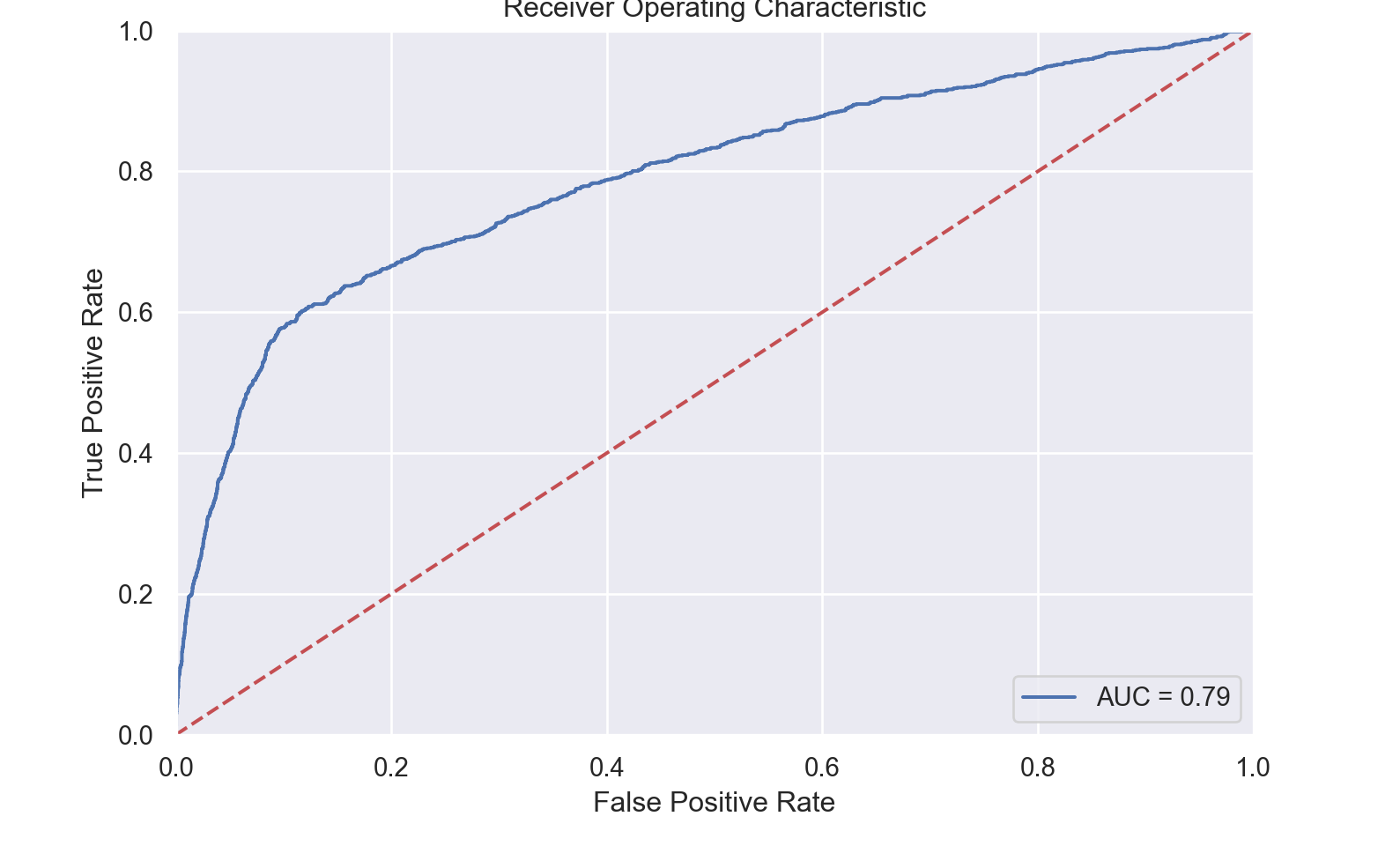

import MLJLinearModels.LogisticClassifier
LinearBinaryClassifier = MLJLinearModels.LogisticClassifier

LogisticClassifier

model = Standardizer |> ContinuousEncoder |> LogisticClassifier

ProbabilisticPipeline(
  standardizer = Standardizer(
        features = Symbol[], 
        ignore = false, 
        ordered_factor = false, 
        count = false), 
  continuous_encoder = ContinuousEncoder(
        drop_last = false, 
        one_hot_ordered_factors = false), 
  logistic_classifier = LogisticClassifier(
        lambda = 2.220446049250313e-16, 
        gamma = 0.0, 
        penalty = :l2, 
        fit_intercept = true, 
        penalize_intercept = false, 
        scale_penalty_with_samples = true, 
        solver = nothing), 
  cache = true)


#tuning = RandomSearch(rng=123);

tuning = Grid(rng=123);

# tuning=LatinHypercube(gens = 1,
#                popsize = 100,
#                ntour = 2,
#                ptour = 0.8,
#                interSampleWeight = 1.0,
#                ae_power = 2,
#                periodic_ae = false,
#                rng=123)

r = range(model,
          :(logistic_classifier.lambda),
          lower=0,
          upper=1,
          unit=0.01)

NumericRange(0 ≤ logistic_classifier.lambda ≤ 1; origin=0.5, unit=0.01)


s = range(model,
          :(logistic_classifier.gamma),
          lower=0,
          upper=1,
          unit=0.01)

NumericRange(0 ≤ logistic_classifier.gamma ≤ 1; origin=0.5, unit=0.01)


tuned_model = TunedModel(model=model,
                         ranges=[r, s],
                         resampling=CV(nfolds=10),
                         measures=auc,
                         tuning=tuning,
                         n=200);

tuned_mach = machine(tuned_model, X_train, y_train);
fit!(tuned_mach);
yhat=MLJ.predict(tuned_mach, X_test);
rep = report(tuned_mach);
print(
    "Measurements:\n",
    "  brier loss: ", brier_loss(yhat,y_test) |> mean, "\n",
    "  auc:        ", auc(yhat,y_test),                "\n",
    "  accuracy:   ", accuracy(mode.(yhat), y_test)
)

Measurements:
  brier loss: 0.16162546559785088
  auc:        0.769700437197346
  accuracy:   0.9018290708967304


# LogisticModel = machine(LinearBinaryClassifierPipe, X_train, y_train);
# fit!(LogisticModel);
# fp = fitted_params(LogisticModel);
# fp.logistic_classifier
#keys(fp)
#rpt = report(LogisticModel)
#keys(rpt)
# fi = rpt.linear_binary_classifier.coef_table |> DataFrames.DataFrame
#ŷ = MLJ.predict(LogisticModel, X_test);
# 
# print(
#     "Measurements:\n",
#     "  brier loss: ", brier_loss(ŷ,y_test) |> mean, "\n",
#     "  auc:        ", auc(ŷ,y_test),                "\n",
#     "  accuracy:   ", accuracy(mode.(ŷ), y_test)
# )
# 
# #confmat(mode.(ŷ),y_test)
# 
# e_pipe = evaluate(LinearBinaryClassifierPipe, X_train, y_train,
#                   resampling=StratifiedCV(nfolds=6, rng=42),
#                   measures=[brier_loss, auc, accuracy],
#                   repeats=1,
#                   acceleration=CPUThreads())


#show(iterated_pipe, 2)

# iterated_pipe = IteratedModel(model=LinearBinaryClassifierPipe,
#                               controls=controls,
#                               measure=auc,
#                               resampling=StratifiedCV(nfolds=6, rng=42))



#mach_iterated_pipe = machine(LinearBinaryClassifierPipe, X_train, y_train);
#fit!(mach_iterated_pipe);
#residuals = [1 - pdf(ŷ[i], y_test[i,1]) for i in 1:nrow(y_test)]
# r = report(LogisticModel)
# 
# k = collect(keys(fp.fitted_params_given_machine))[3]
# println("\n Coefficients:  ", fp.fitted_params_given_machine[k].coef)
# println("\n y \n ", y_test[1:5,1])
# println("\n ŷ \n ", ŷ[1:5])
# println("\n residuals \n ", residuals[1:5])
# println("\n Standard Error per Coefficient \n", r.linear_binary_classifier.stderror[2:end])


#confusion_matrix(yMode, y_test)

Naive Bayes

nb_recipe <- 
  recipe(formula = y ~ ., data = data_bank_marketing_train) %>%
  step_rm(duration) %>% 
  step_dummy()

nb_spec <- 
  naive_Bayes(smoothness = tune(), Laplace = tune()) %>%
  set_engine("naivebayes")

nb_workflow <- 
  workflow() %>% 
  add_recipe(nb_recipe) %>% 
  add_model(nb_spec)

#nb_params = extract_parameter_set_dials(nb_spec)

# nb_grid = nb_params %>% grid_latin_hypercube(size = 20, original = FALSE)
# 
# nb_tune <-
#   nb_workflow %>%
#   tune_grid(
#     data_folds,
#     grid = nb_grid
#   )
# nb_tune
# select_best(nb_tune, metric = "roc_auc")

final_params = tibble(
                smoothness = 0.5923033,
                Laplace = 0.4830422
              )

final_nb_wflow <- 
  nb_workflow %>% 
  finalize_workflow(final_params)

final_nb_fit <- 
  final_nb_wflow %>% 
  last_fit(data_bank_marketing_split)

final_nb_fit %>% collect_metrics()

# A tibble: 2 × 4
  .metric  .estimator .estimate .config             
  <chr>    <chr>          <dbl> <chr>               
1 accuracy binary         0.880 Preprocessor1_Model1
2 roc_auc  binary         0.795 Preprocessor1_Model1

final_nb_fit %>% collect_predictions()

# A tibble: 10,297 × 7
   id               .pred_no   .pred_yes  .row .pred_class y     .config        
   <chr>               <dbl>       <dbl> <int> <fct>       <fct> <chr>          
 1 train/test split     1.00 0.00000488      7 no          no    Preprocessor1_…
 2 train/test split     1.00 0.000000414    18 no          no    Preprocessor1_…
 3 train/test split     1.00 0.00000451     21 no          no    Preprocessor1_…
 4 train/test split     1.00 0.000000644    22 no          no    Preprocessor1_…
 5 train/test split     1.00 0.00000345     24 no          no    Preprocessor1_…
 6 train/test split     1.00 0.000000957    30 no          no    Preprocessor1_…
 7 train/test split     1.00 0.00000110     34 no          no    Preprocessor1_…
 8 train/test split     1.00 0.00000159     35 no          no    Preprocessor1_…
 9 train/test split     1.00 0.00000488     43 no          no    Preprocessor1_…
10 train/test split     1.00 0.00000200     52 no          no    Preprocessor1_…
# … with 10,287 more rows

final_nb_fit %>% collect_predictions() %>% roc_curve(y, .pred_no) %>% autoplot()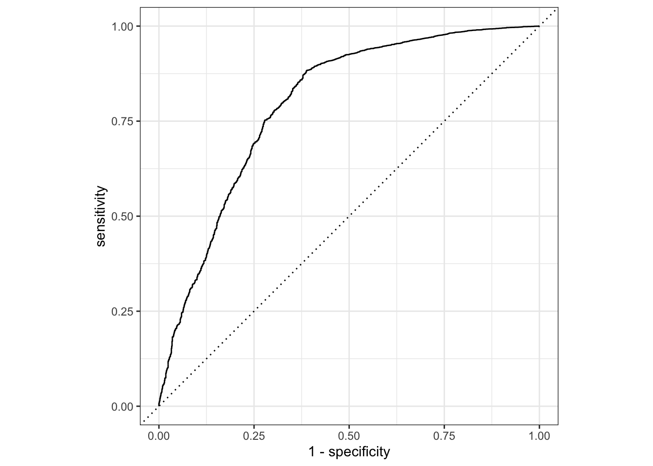

nb_auc = final_nb_fit %>% collect_predictions() %>% roc_curve(y, .pred_no) %>% mutate(model = "naive bayes")

model = GaussianNB()

model.fit(X_trans_train, y_trans_train)

GaussianNB()

model.predict_proba(X_trans_test)

array([[9.99990953e-01, 9.04749432e-06],
       [8.12354222e-01, 1.87645778e-01],
       [9.99999789e-01, 2.10792883e-07],
       ...,
       [9.99294556e-01, 7.05443805e-04],
       [9.99995515e-01, 4.48497521e-06],
       [7.16817215e-01, 2.83182785e-01]])

roc_plot(X_trans_test, y_trans_test, model, 1)

0.7567412601500412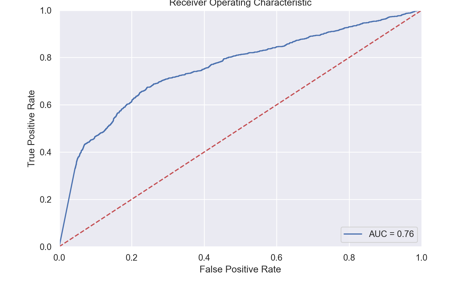

import NaiveBayes

GaussianNBClassifier = @load GaussianNBClassifier pkg=NaiveBayes;

model = Standardizer |> ContinuousEncoder |> GaussianNBClassifier()

ProbabilisticPipeline(
  standardizer = Standardizer(
        features = Symbol[], 
        ignore = false, 
        ordered_factor = false, 
        count = false), 
  continuous_encoder = ContinuousEncoder(
        drop_last = false, 
        one_hot_ordered_factors = false), 
  gaussian_nb_classifier = GaussianNBClassifier(), 
  cache = true)


# Model training fails with error: nested task error: PosDefException: matrix is not positive definite; Cholesky factorization failed.
# Pre-processing to eliminate collinearity may be needed

# mach = machine(model, X_train, y_train);
# 
# fit!(mach);
# yhat=MLJ.predict(mach, X_test);
# rep = report(mach);
# print(
#     "Measurements:\n",
#     "  brier loss: ", brier_loss(yhat,y_test) |> mean, "\n",
#     "  auc:        ", auc(yhat,y_test),                "\n",
#     "  accuracy:   ", accuracy(mode.(yhat), y_test)
# )

KNN

#use_kknn(y ~ ., data = data_bank_marketing_train)
kknn_recipe <-
  recipe(formula = y ~ ., data = data_bank_marketing_train) %>%
  step_rm(duration) %>% 
  step_string2factor(one_of("job", "marital", "education", "default", "housing",
    "loan", "contact", "month", "day_of_week", "poutcome", "y")) %>%
  step_novel(all_nominal_predictors()) %>%
  step_dummy(all_nominal_predictors()) %>%
  step_zv(all_predictors()) %>%
  step_normalize(all_numeric_predictors())

kknn_spec <-
  nearest_neighbor(neighbors = tune()) %>%
  set_mode("classification") %>%
  set_engine("kknn")

kknn_param = extract_parameter_set_dials(kknn_spec)

kknn_workflow <-
  workflow() %>%
  add_recipe(kknn_recipe) %>%
  add_model(kknn_spec)

set.seed(66214)
# kknn_tune <-
#   tune_grid(kknn_workflow, resamples = data_folds, size =10)

final_params <-
  tibble(
    neighbors = 14
  )

final_kknn_wflow = kknn_workflow %>% finalize_workflow(final_params)
final_kknn_wflow

══ Workflow ════════════════════════════════════════════════════════════════════
Preprocessor: Recipe
Model: nearest_neighbor()

── Preprocessor ────────────────────────────────────────────────────────────────
6 Recipe Steps

• step_rm()
• step_string2factor()
• step_novel()
• step_dummy()
• step_zv()
• step_normalize()

── Model ───────────────────────────────────────────────────────────────────────
K-Nearest Neighbor Model Specification (classification)

Main Arguments:
  neighbors = 14

Computational engine: kknn

final_kknn_fit = final_kknn_wflow %>% last_fit(data_bank_marketing_split)

final_kknn_fit %>% collect_metrics()

# A tibble: 2 × 4
  .metric  .estimator .estimate .config             
  <chr>    <chr>          <dbl> <chr>               
1 accuracy binary         0.894 Preprocessor1_Model1
2 roc_auc  binary         0.751 Preprocessor1_Model1

final_kknn_fit %>% collect_predictions()

# A tibble: 10,297 × 7
   id               .pred_no .pred_yes  .row .pred_class y     .config          
   <chr>               <dbl>     <dbl> <int> <fct>       <fct> <chr>            
 1 train/test split    1        0          7 no          no    Preprocessor1_Mo…
 2 train/test split    0.932    0.0682    18 no          no    Preprocessor1_Mo…
 3 train/test split    1        0         21 no          no    Preprocessor1_Mo…
 4 train/test split    0.932    0.0682    22 no          no    Preprocessor1_Mo…
 5 train/test split    1        0         24 no          no    Preprocessor1_Mo…
 6 train/test split    1        0         30 no          no    Preprocessor1_Mo…
 7 train/test split    0.749    0.251     34 no          no    Preprocessor1_Mo…
 8 train/test split    1        0         35 no          no    Preprocessor1_Mo…
 9 train/test split    1        0         43 no          no    Preprocessor1_Mo…
10 train/test split    1        0         52 no          no    Preprocessor1_Mo…
# … with 10,287 more rows

final_kknn_fit %>% collect_predictions() %>% roc_curve(y, .pred_no) %>% autoplot()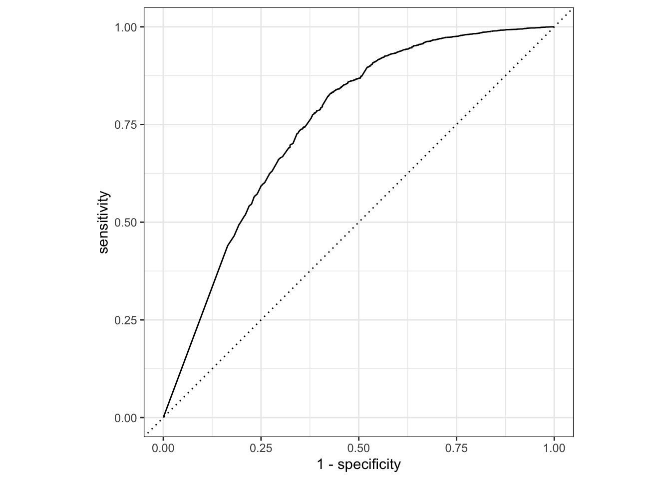

kknn_auc = final_kknn_fit %>% collect_predictions() %>% roc_curve(y, .pred_no) %>% mutate(model = "knn")

model = KNeighborsClassifier()
param_grid = {'model__n_neighbors':np.arange(0,20,1)}

steps[-1] = ("model", model)

pipe = Pipeline(steps)

grid = GridSearchCV(pipe, param_grid, cv=10, scoring='roc_auc')

grid.fit(data_bank_marketing_train, y_train)

grid.best_params_

{'model__n_neighbors': 19}

fitted_model=grid.best_estimator_
score=grid.score(data_bank_marketing_test, y_test)
score

0.7583868296985286

yhat=grid.predict(data_bank_marketing_test)

roc_plot(data_bank_marketing_test, y_test, fitted_model, 'yes')

0.7583868296985286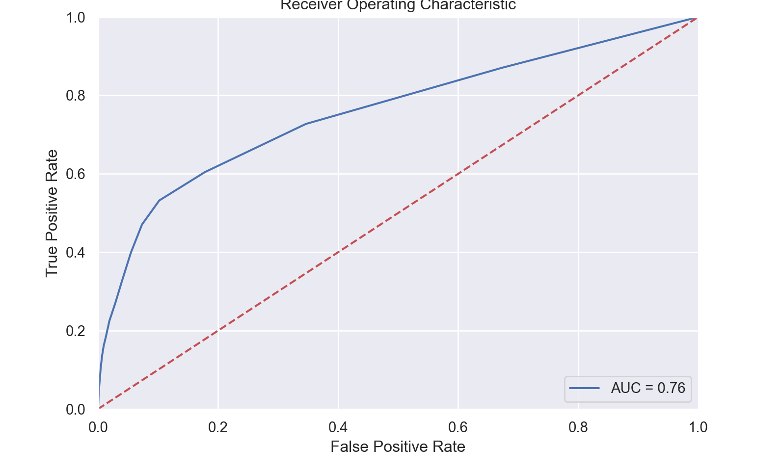

import NearestNeighborModels
KNNClassifier = @load KNNClassifier pkg=NearestNeighborModels verbosity=0

NearestNeighborModels.KNNClassifier


model = Standardizer |> ContinuousEncoder |> KNNClassifier()

ProbabilisticPipeline(
  standardizer = Standardizer(
        features = Symbol[], 
        ignore = false, 
        ordered_factor = false, 
        count = false), 
  continuous_encoder = ContinuousEncoder(
        drop_last = false, 
        one_hot_ordered_factors = false), 
  knn_classifier = KNNClassifier(
        K = 5, 
        algorithm = :kdtree, 
        metric = Distances.Euclidean(0.0), 
        leafsize = 10, 
        reorder = true, 
        weights = NearestNeighborModels.Uniform()), 
  cache = true)


mach = machine(model, X_train, y_train);

fit!(mach);
yhat=MLJ.predict(mach, X_test);
rep = report(mach);
print(
    "Measurements:\n",
    "  brier loss: ", brier_loss(yhat,y_test) |> mean, "\n",
    "  auc:        ", auc(yhat,y_test),                "\n",
    "  accuracy:   ", accuracy(mode.(yhat), y_test)
)

Measurements:
  brier loss: 0.1816056976367755
  auc:        0.7262961939438142
  accuracy:   0.8910650696018129


#doc("KNNClassifier", pkg="NearestNeighborModels")

Support Vector Machine

svm_spec = svm_rbf(cost = 1, margin = 0.1) %>%
                set_mode("classification") %>%
                set_engine("kernlab")

base_rec = recipe(y ~ ., data = data_bank_marketing_train) %>% step_rm(duration) %>%
            step_zv(all_numeric_predictors()) %>%
            step_normalize(all_numeric_predictors())

svm_rec = base_rec %>%
            step_dummy(all_nominal_predictors())
svm_data = prep(svm_rec, data_bank_marketing_train) %>% bake(new_data = NULL)

svm_wrkflw = workflow() %>% add_model(svm_spec) %>% add_recipe(svm_rec)
svm_wrkflw

══ Workflow ════════════════════════════════════════════════════════════════════
Preprocessor: Recipe
Model: svm_rbf()

── Preprocessor ────────────────────────────────────────────────────────────────
4 Recipe Steps

• step_rm()
• step_zv()
• step_normalize()
• step_dummy()

── Model ───────────────────────────────────────────────────────────────────────
Radial Basis Function Support Vector Machine Model Specification (classification)

Main Arguments:
  cost = 1
  margin = 0.1

Computational engine: kernlab

grid_ctrl <-
   control_grid (
      save_pred = TRUE,
      parallel_over = "everything",
      save_workflow = TRUE
   )

final_svm_fit = svm_wrkflw %>% fit(data=data_bank_marketing_train)

final_svm_pred = final_svm_fit %>% predict(data_bank_marketing_test, type = "prob")
final_svm_pred = final_svm_pred %>% cbind(data_bank_marketing_test %>% select(y))
final_svm_pred$y = as.factor(final_svm_pred$y)

final_svm_pred %>%  roc_curve(y, .pred_no) %>% autoplot()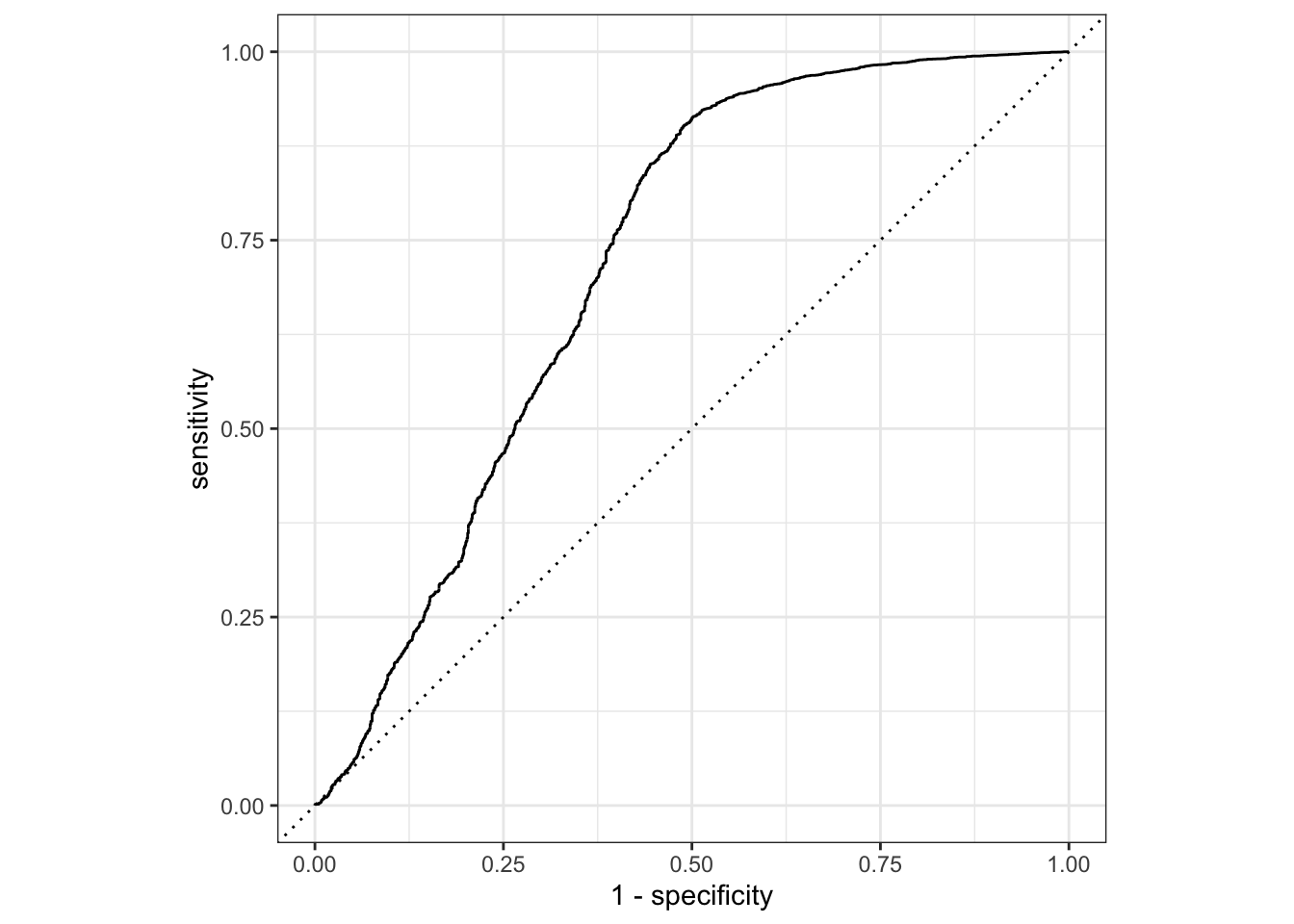

svm_auc = final_svm_pred %>%  roc_curve(y, .pred_no) %>% mutate(model="svm")

# Cross validation\ grid search is not used for SVC as it is too slow due to the 40K+ observations and 19 features.
model = SVC(kernel='rbf', C=1, gamma = 0.1, probability=True)

# Remove the previous model; the pipeline in this case is used only for data transformation and not model fitting
steps.pop()

# transform train data

('model', KNeighborsClassifier())

X_trans_train = pipe.fit_transform(data_bank_marketing_train, y_train)

# transform y
label_encoder = LabelEncoder()
y_trans_train = label_encoder.fit_transform(y_train)
y_trans_test = label_encoder.fit_transform(y_test)

# model needs to be fit first due to 'prefit' option used for CalibratedClassifierCV
model.fit(X_trans_train, y_trans_train)

# CalibratedClassifierCV is used to find probabilities, and not for cross validation

SVC(C=1, gamma=0.1, probability=True)

calibrated_clf = CalibratedClassifierCV(model, cv = 'prefit')

# fit again to find probabilities
calibrated_clf.fit(X_trans_train, y_trans_train)

CalibratedClassifierCV(cv='prefit',
                       estimator=SVC(C=1, gamma=0.1, probability=True))

calibrated_clf.predict_proba(X_trans_train)

# transform test data

array([[0.9119843 , 0.0880157 ],
       [0.9120593 , 0.0879407 ],
       [0.91198241, 0.08801759],
       ...,
       [0.91272997, 0.08727003],
       [0.9137733 , 0.0862267 ],
       [0.91701637, 0.08298363]])

X_trans_test = pipe.fit_transform(data_bank_marketing_test, y_test)
yhat = calibrated_clf.predict(X_trans_test)

report=metrics.classification_report(y_trans_test,yhat)
print(report)

              precision    recall  f1-score   support

           0       0.91      0.99      0.94      9139
           1       0.65      0.19      0.29      1158

    accuracy                           0.90     10297
   macro avg       0.78      0.59      0.62     10297
weighted avg       0.88      0.90      0.87     10297

roc_plot(X_trans_test, y_trans_test, model, 1)

0.71219394910423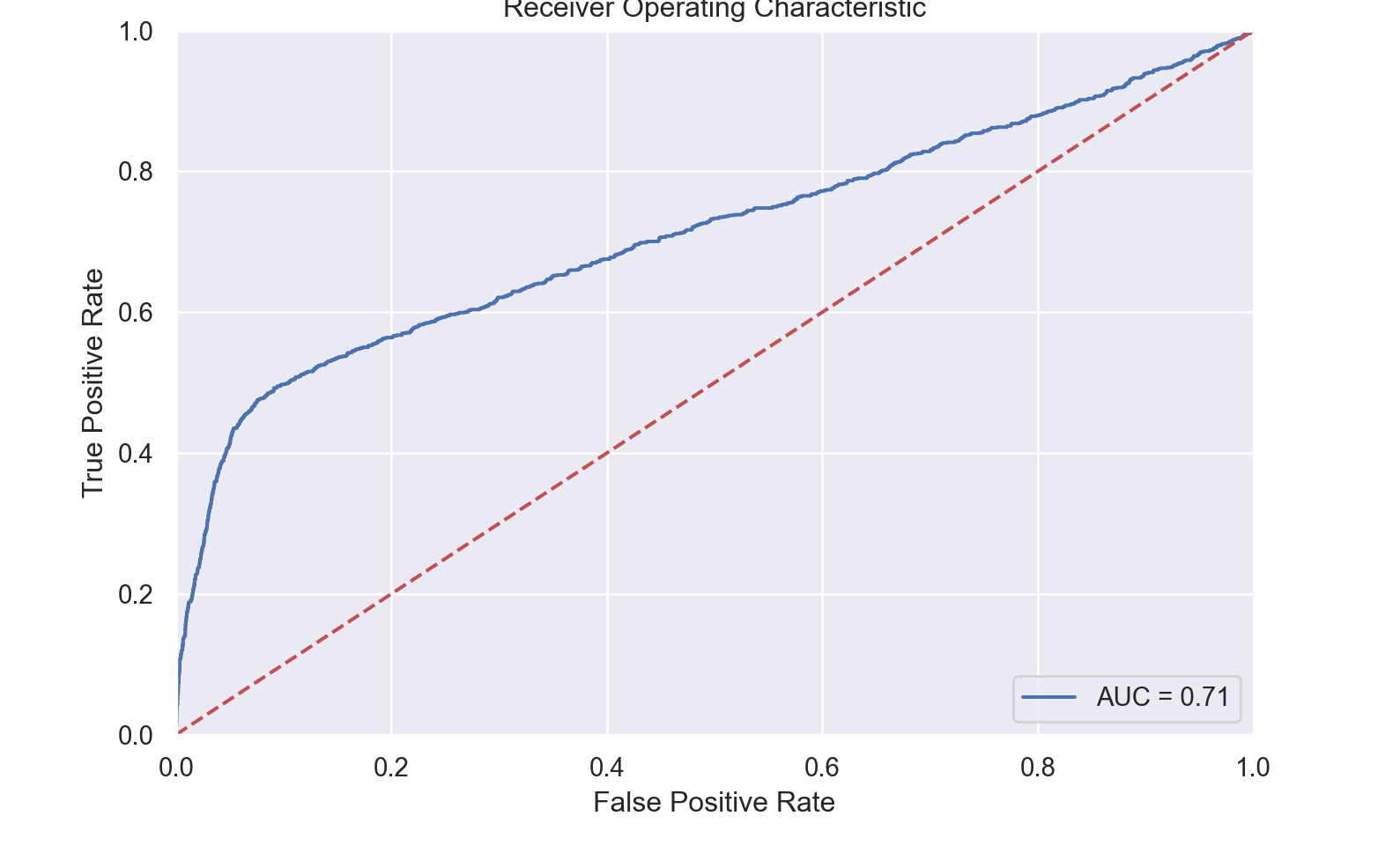

import LIBSVM
#doc("ProbabilisticSVC", pkg="LIBSVM")
ProbabilisticSVC = @load ProbabilisticSVC pkg=LIBSVM verbosity=0

MLJLIBSVMInterface.ProbabilisticSVC


model = Standardizer |> ContinuousEncoder |> ProbabilisticSVC(kernel=LIBSVM.Kernel.RadialBasis, gamma = 0.1)

ProbabilisticPipeline(
  standardizer = Standardizer(
        features = Symbol[], 
        ignore = false, 
        ordered_factor = false, 
        count = false), 
  continuous_encoder = ContinuousEncoder(
        drop_last = false, 
        one_hot_ordered_factors = false), 
  probabilistic_svc = ProbabilisticSVC(
        kernel = LIBSVM.Kernel.RadialBasis, 
        gamma = 0.1, 
        cost = 1.0, 
        cachesize = 200.0, 
        degree = 3, 
        coef0 = 0.0, 
        tolerance = 0.001, 
        shrinking = true), 
  cache = true)


mach = machine(model, X_train, y_train);

fit!(mach);
yhat=MLJ.predict(mach, X_test);
rep = report(mach);
print(
    "Measurements:\n",
    "  brier loss: ", brier_loss(yhat,y_test) |> mean, "\n",
    "  auc:        ", auc(yhat,y_test),                "\n",
    "  accuracy:   ", accuracy(mode.(yhat), y_test)
)

Measurements:
  brier loss: 0.16360023292036047
  auc:        0.7202998911144449
  accuracy:   0.901181612172224

XGBoost

xgboost_recipe =
  recipe(formula = y ~ ., data = data_bank_marketing_train) %>%
  step_rm(duration) %>%
  ## For modeling, it is preferred to encode qualitative data as factors
  ## (instead of character).
  step_string2factor(one_of("job", "marital", "education", "default", "housing",
    "loan", "contact", "month", "day_of_week", "poutcome", "y")) %>%
  step_novel(all_nominal_predictors()) %>%
  ## This model requires the predictors to be numeric. The most common
  ## method to convert qualitative predictors to numeric is to create
  ## binary indicator variables (aka dummy variables) from these
  ## predictors. However, for this model, binary indicator variables can be
  ## made for each of the levels of the factors (known as 'one-hot
  ## encoding').
  step_dummy(all_nominal_predictors(), one_hot = TRUE) %>%
  step_zv(all_predictors())

xgboost_spec =
  boost_tree(trees = tune(), tree_depth = tune(), learn_rate = tune(), loss_reduction = tune(), min_n = tune(), sample_size = tune()) %>%
  set_mode("classification") %>%
  set_engine("xgboost")

xgboost_workflow =
  workflow() %>%
  add_recipe(xgboost_recipe) %>%
  add_model(xgboost_spec)

xgboost_param <- extract_parameter_set_dials(xgboost_spec)

set.seed(87274)
final_params <-
  tibble(
    trees = 1453,
    tree_depth = 11,
    learn_rate = 0.052975,
    loss_reduction = 7.733554,
    min_n = 26,
    sample_size = 0.9654255
  )

final_xgboost_wflow = xgboost_workflow %>% finalize_workflow(final_params)
final_xgboost_wflow

══ Workflow ════════════════════════════════════════════════════════════════════
Preprocessor: Recipe
Model: boost_tree()

── Preprocessor ────────────────────────────────────────────────────────────────
5 Recipe Steps

• step_rm()
• step_string2factor()
• step_novel()
• step_dummy()
• step_zv()

── Model ───────────────────────────────────────────────────────────────────────
Boosted Tree Model Specification (classification)

Main Arguments:
  trees = 1453
  min_n = 26
  tree_depth = 11
  learn_rate = 0.052975
  loss_reduction = 7.733554
  sample_size = 0.9654255

Computational engine: xgboost

final_xgboost_fit = final_xgboost_wflow %>% last_fit(data_bank_marketing_split)

final_xgboost_fit %>% collect_metrics()

# A tibble: 2 × 4
  .metric  .estimator .estimate .config             
  <chr>    <chr>          <dbl> <chr>               
1 accuracy binary         0.901 Preprocessor1_Model1
2 roc_auc  binary         0.816 Preprocessor1_Model1

final_xgboost_fit %>% collect_predictions()

# A tibble: 10,297 × 7
   id               .pred_no .pred_yes  .row .pred_class y     .config          
   <chr>               <dbl>     <dbl> <int> <fct>       <fct> <chr>            
 1 train/test split    0.971    0.0286     7 no          no    Preprocessor1_Mo…
 2 train/test split    0.973    0.0274    18 no          no    Preprocessor1_Mo…
 3 train/test split    0.974    0.0257    21 no          no    Preprocessor1_Mo…
 4 train/test split    0.978    0.0222    22 no          no    Preprocessor1_Mo…
 5 train/test split    0.970    0.0305    24 no          no    Preprocessor1_Mo…
 6 train/test split    0.979    0.0212    30 no          no    Preprocessor1_Mo…
 7 train/test split    0.977    0.0230    34 no          no    Preprocessor1_Mo…
 8 train/test split    0.976    0.0240    35 no          no    Preprocessor1_Mo…
 9 train/test split    0.973    0.0267    43 no          no    Preprocessor1_Mo…
10 train/test split    0.979    0.0210    52 no          no    Preprocessor1_Mo…
# … with 10,287 more rows

final_xgboost_fit %>% collect_predictions() %>% roc_curve(y, .pred_no) %>% autoplot()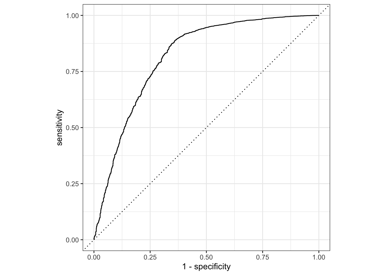

xgboost_auc = final_xgboost_fit %>% collect_predictions() %>% roc_curve(y, .pred_no) %>% mutate(model = "xgboost")


from sklearn.model_selection import StratifiedKFold
from xgboost import XGBClassifier

def grid_search_xgb(params, X, y, kfold, random=False):

  xgb = XGBClassifier(booster='gbtree', objective='binary:logistic', random_state=2)
  if random:
    grid = RandomizedSearchCV(xgb, params, cv=kfold, n_iter=10, n_jobs=-1, scoring='roc_auc') #n_iter controls number of random combinations
  else:
    grid = GridSearchCV(xgb, params, cv=kfold,n_jobs=-1, scoring='roc_auc')

  grid.fit(X, y)

  print('Best params:', grid.best_params_)
  print('Best score:', grid.best_score_)
#
#
st_Kfold = StratifiedKFold(n_splits=5, shuffle=True, random_state=2)
#
# #n_estimators is the number of trees trained, default is 100. 7 seems to be an optimum value.
# params={'n_estimators':[7,10]}
# grid_search_xgb(params, X_trans_train, y_trans_train, st_Kfold)
#
# #learning_rate shrinks the weights of trees for each round of boosting, default is 0.3. By lowering learning_rate, more trees are required to produce better scores. Lowering learning_rate prevents overﬁtting because the size of the weights carried forward is smaller. 0.05 seems to be an optimum value.
# params={'learning_rate':[0.01, 0.05, 0.075, 0.1, 0.2, 0.3, 0.4, 0.5]}
# grid_search_xgb(params, X_trans_train, y_trans_train, st_Kfold)
#
# #max_depth determines the length of the tree, equivalent to the number of rounds of splitting. default is 6. Limiting max_depth prevents overﬁtting because the individual trees can only grow as far as max_depth allows. 2 seems to be an optimum value.
# params={'max_depth':[1,2, 3, 5, 6, 8]}
# grid_search_xgb(params, X_trans_train, y_trans_train, st_Kfold)
#
# #gamma provides a threshold that nodes must surpass before making further splits according to the loss function, default is 0.There is no upper limit to the value of gamma. Anything over 10 is considered very high. Increasing gamma results in a more conservative model. 5 seems to be an optimum value.
# params={'gamma':[0, 0.1, 0.5, 1, 2, 5, 7]}
# grid_search_xgb(params, X_trans_train, y_trans_train, st_Kfold)
#
# #min_child_weight refers to the minimum sum of weights required for a node to split into a child. If the sum of the weights is less than the value of min_child_weight, no further splits are made.min_child_weight reduces overﬁtting by increasing its value. 4 seems to be an optimum value.
# params={'min_child_weight':[1, 2, 3, 4, 5]}
# grid_search_xgb(params, X_trans_train, y_trans_train, st_Kfold)
#
# #The subsample hyperparameter limits the percentage of training instances (rows) for each boosting round. Decreasing subsample from 100% reduces overﬁtting. 1 seems to be an optimum value:
# params={'subsample':[0.5, 0.7, 0.8, 0.9, 1]}
# grid_search_xgb(params, X_trans_train, y_trans_train, st_Kfold)
#
# #colsample_bytree randomly selects particular columnsaccording to the given percentage.colsample_bytree is useful for limiting the inﬂuence of columns and reducing variance. 0.7 seems to be an optimum value.
# params={'colsample_bytree':[0.5, 0.7, 0.8, 0.9,1]}
# grid_search_xgb(params, X_trans_train, y_trans_train, st_Kfold)
#
#
params={'n_estimators':[5,7,10,20,50],
        'learning_rate': [0.05,0.1, 0.2, 0.3, 0.4, 0.5],
        'max_depth': [2,4,6],
        'gamma': [0.1,0.5,2, 5],
        'min_child_weight': [3,4,5],
        'subsample': [0.5,1],
        'colsample_bytree': [0.5,0.7,1]}
# # ->grid_search_xgb(params, X_trans_train, y_trans_train, st_Kfold)
#
#
# #Output:
# #Best params: {'colsample_bytree': 0.7, 'gamma': 0.1, 'learning_rate': 0.1, 'max_depth': 6, 'min_child_weight': 4, 'n_estimators': 50, 'subsample': 1}
# #Best score: 0.800812151928098
#
#
params={'n_estimators':[20,50,75,100],
        'learning_rate': [0.05,0.1, 0.15, 0.2],
        'max_depth': [6,8,10],
        'gamma': [0.1,0.2,0.3],
        'min_child_weight': [3,4,5],
        'subsample': [0.75,1],
        'colsample_bytree': [0.7,0.8,1]}
#
# # ->grid_search_xgb(params, X_trans_train, y_trans_train, st_Kfold, random=True)
#
# # ->grid_search(params={'subsample':[0.5, 0.6, 0.7, 0.8, 0.9, 1],'min_child_weight':[1, 2, 3, 4, 5],'learning_rate':[0.1, 0.2, 0.3, 0.4, 0.5],'max_depth':[1, 2, 3, 4, 5], 'n_estimators':[2]})
# #Best params: {'subsample': 1, 'n_estimators': 75, 'min_child_weight': 3, 'max_depth': 8, 'learning_rate': 0.05, 'gamma': 0.1, 'colsample_bytree': 0.7}
# #Best score: 0.8013732623090342
#
final_model = XGBClassifier(booster='gbtree',objective='binary:logistic', max_depth=8, learning_rate=0.05, n_estimators=75, subsample=1, min_child_weight=3, gamma=0.1, colsample_bytree=0.7, random_state=2, n_jobs=-1)
#
fitted_model=final_model.fit(X_trans_train, y_trans_train)
print ('ROC AUC Score',roc_plot(X_trans_test,y_trans_test, fitted_model, 1))

ROC AUC Score 0.8105681566276057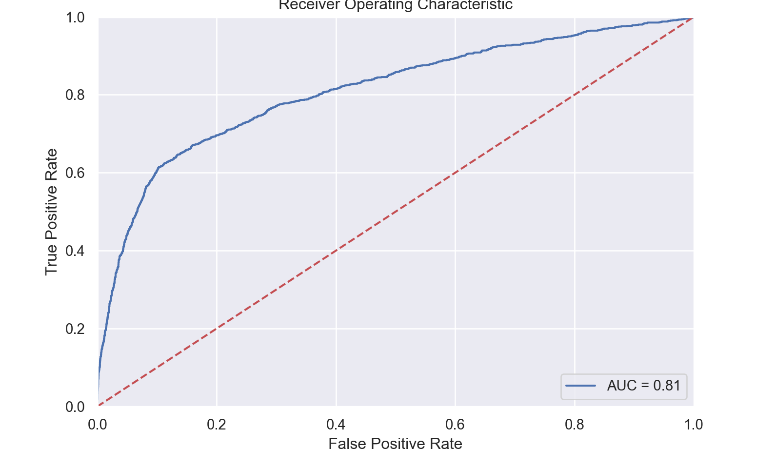

XGBoostClassifier = @load XGBoostClassifier pkg=XGBoost verbosity=0

MLJXGBoostInterface.XGBoostClassifier


model = Standardizer |> ContinuousEncoder |> XGBoostClassifier

ProbabilisticPipeline(
  standardizer = Standardizer(
        features = Symbol[], 
        ignore = false, 
        ordered_factor = false, 
        count = false), 
  continuous_encoder = ContinuousEncoder(
        drop_last = false, 
        one_hot_ordered_factors = false), 
  xg_boost_classifier = XGBoostClassifier(
        test = 1, 
        num_round = 100, 
        booster = "gbtree", 
        disable_default_eval_metric = 0, 
        eta = 0.3, 
        num_parallel_tree = 1, 
        gamma = 0.0, 
        max_depth = 6, 
        min_child_weight = 1.0, 
        max_delta_step = 0.0, 
        subsample = 1.0, 
        colsample_bytree = 1.0, 
        colsample_bylevel = 1.0, 
        colsample_bynode = 1.0, 
        lambda = 1.0, 
        alpha = 0.0, 
        tree_method = "auto", 
        sketch_eps = 0.03, 
        scale_pos_weight = 1.0, 
        updater = nothing, 
        refresh_leaf = 1, 
        process_type = "default", 
        grow_policy = "depthwise", 
        max_leaves = 0, 
        max_bin = 256, 
        predictor = "cpu_predictor", 
        sample_type = "uniform", 
        normalize_type = "tree", 
        rate_drop = 0.0, 
        one_drop = 0, 
        skip_drop = 0.0, 
        feature_selector = "cyclic", 
        top_k = 0, 
        tweedie_variance_power = 1.5, 
        objective = "automatic", 
        base_score = 0.5, 
        watchlist = nothing, 
        nthread = 1, 
        importance_type = "gain", 
        seed = nothing, 
        validate_parameters = false), 
  cache = true)

show(model, 2)

ProbabilisticPipeline(
  standardizer = Standardizer(
        features = Symbol[], 
        ignore = false, 
        ordered_factor = false, 
        count = false), 
  continuous_encoder = ContinuousEncoder(
        drop_last = false, 
        one_hot_ordered_factors = false), 
  xg_boost_classifier = XGBoostClassifier(
        test = 1, 
        num_round = 100, 
        booster = "gbtree", 
        disable_default_eval_metric = 0, 
        eta = 0.3, 
        num_parallel_tree = 1, 
        gamma = 0.0, 
        max_depth = 6, 
        min_child_weight = 1.0, 
        max_delta_step = 0.0, 
        subsample = 1.0, 
        colsample_bytree = 1.0, 
        colsample_bylevel = 1.0, 
        colsample_bynode = 1.0, 
        lambda = 1.0, 
        alpha = 0.0, 
        tree_method = "auto", 
        sketch_eps = 0.03, 
        scale_pos_weight = 1.0, 
        updater = nothing, 
        refresh_leaf = 1, 
        process_type = "default", 
        grow_policy = "depthwise", 
        max_leaves = 0, 
        max_bin = 256, 
        predictor = "cpu_predictor", 
        sample_type = "uniform", 
        normalize_type = "tree", 
        rate_drop = 0.0, 
        one_drop = 0, 
        skip_drop = 0.0, 
        feature_selector = "cyclic", 
        top_k = 0, 
        tweedie_variance_power = 1.5, 
        objective = "automatic", 
        base_score = 0.5, 
        watchlist = nothing, 
        nthread = 1, 
        importance_type = "gain", 
        seed = nothing, 
        validate_parameters = false), 
  cache = true)

#models("xgboost")
XGBoostClassifier = @load XGBoostClassifier pkg=XGBoost

import MLJXGBoostInterface ✔

MLJXGBoostInterface.XGBoostClassifier


model = Standardizer |> ContinuousEncoder |> XGBoostClassifier

ProbabilisticPipeline(
  standardizer = Standardizer(
        features = Symbol[], 
        ignore = false, 
        ordered_factor = false, 
        count = false), 
  continuous_encoder = ContinuousEncoder(
        drop_last = false, 
        one_hot_ordered_factors = false), 
  xg_boost_classifier = XGBoostClassifier(
        test = 1, 
        num_round = 100, 
        booster = "gbtree", 
        disable_default_eval_metric = 0, 
        eta = 0.3, 
        num_parallel_tree = 1, 
        gamma = 0.0, 
        max_depth = 6, 
        min_child_weight = 1.0, 
        max_delta_step = 0.0, 
        subsample = 1.0, 
        colsample_bytree = 1.0, 
        colsample_bylevel = 1.0, 
        colsample_bynode = 1.0, 
        lambda = 1.0, 
        alpha = 0.0, 
        tree_method = "auto", 
        sketch_eps = 0.03, 
        scale_pos_weight = 1.0, 
        updater = nothing, 
        refresh_leaf = 1, 
        process_type = "default", 
        grow_policy = "depthwise", 
        max_leaves = 0, 
        max_bin = 256, 
        predictor = "cpu_predictor", 
        sample_type = "uniform", 
        normalize_type = "tree", 
        rate_drop = 0.0, 
        one_drop = 0, 
        skip_drop = 0.0, 
        feature_selector = "cyclic", 
        top_k = 0, 
        tweedie_variance_power = 1.5, 
        objective = "automatic", 
        base_score = 0.5, 
        watchlist = nothing, 
        nthread = 1, 
        importance_type = "gain", 
        seed = nothing, 
        validate_parameters = false), 
  cache = true)

show(model, 2)

ProbabilisticPipeline(
  standardizer = Standardizer(
        features = Symbol[], 
        ignore = false, 
        ordered_factor = false, 
        count = false), 
  continuous_encoder = ContinuousEncoder(
        drop_last = false, 
        one_hot_ordered_factors = false), 
  xg_boost_classifier = XGBoostClassifier(
        test = 1, 
        num_round = 100, 
        booster = "gbtree", 
        disable_default_eval_metric = 0, 
        eta = 0.3, 
        num_parallel_tree = 1, 
        gamma = 0.0, 
        max_depth = 6, 
        min_child_weight = 1.0, 
        max_delta_step = 0.0, 
        subsample = 1.0, 
        colsample_bytree = 1.0, 
        colsample_bylevel = 1.0, 
        colsample_bynode = 1.0, 
        lambda = 1.0, 
        alpha = 0.0, 
        tree_method = "auto", 
        sketch_eps = 0.03, 
        scale_pos_weight = 1.0, 
        updater = nothing, 
        refresh_leaf = 1, 
        process_type = "default", 
        grow_policy = "depthwise", 
        max_leaves = 0, 
        max_bin = 256, 
        predictor = "cpu_predictor", 
        sample_type = "uniform", 
        normalize_type = "tree", 
        rate_drop = 0.0, 
        one_drop = 0, 
        skip_drop = 0.0, 
        feature_selector = "cyclic", 
        top_k = 0, 
        tweedie_variance_power = 1.5, 
        objective = "automatic", 
        base_score = 0.5, 
        watchlist = nothing, 
        nthread = 1, 
        importance_type = "gain", 
        seed = nothing, 
        validate_parameters = false), 
  cache = true)

tuning = RandomSearch(rng=123);

eta = range(model,
          :(xg_boost_classifier.eta),
          lower=0.1,
          upper=1,
          unit=0.2)

NumericRange(0.1 ≤ xg_boost_classifier.eta ≤ 1.0; origin=0.55, unit=0.2)


gamma = range(model,
          :(xg_boost_classifier.gamma),
          lower=1,
          upper=6,
          unit=1)

NumericRange(1.0 ≤ xg_boost_classifier.gamma ≤ 6.0; origin=3.5, unit=1.0)


max_depth = range(model,
          :(xg_boost_classifier.max_depth),
          lower=1,
          upper=6,
          unit=1)

NumericRange(1 ≤ xg_boost_classifier.max_depth ≤ 6; origin=3.5, unit=1.0)


subsample = range(model,
          :(xg_boost_classifier.subsample),
          lower=0.1,
          upper=1,
          unit=0.25)

NumericRange(0.1 ≤ xg_boost_classifier.subsample ≤ 1.0; origin=0.55, unit=0.25)


colsample_bytree = range(model,
          :(xg_boost_classifier.colsample_bytree),
          lower=0.2,
          upper=1,
          unit=0.25)

NumericRange(0.2 ≤ xg_boost_classifier.colsample_bytree ≤ 1.0; origin=0.6, unit=0.25)


tuned_model = TunedModel(model=model,
                         ranges=[eta, gamma, max_depth,subsample,colsample_bytree],
                         resampling=CV(nfolds=10),
                         measures=auc,
                         tuning=tuning,
                         n=50);

mach = machine(tuned_model, X_train, y_train);

fit!(mach);
yhat=MLJ.predict(mach, X_test);
rep = report(mach);
print(
    "Measurements:\n",
    "  brier loss: ", brier_loss(yhat,y_test) |> mean, "\n",
    "  auc:        ", auc(yhat,y_test),                "\n",
    "  accuracy:   ", accuracy(mode.(yhat), y_test)
)

Measurements:
  brier loss: 0.1494576
  auc:        0.8101407168755788
  accuracy:   0.9040142440919392


#Results for n=50
#brier loss: 0.1494576
#auc:        0.8101407168755788
#accuracy:   0.9040142440919392

println(rep.best_model.xg_boost_classifier.eta) # 0.2835969604842409

0.2835969604842409

println(rep.best_model.xg_boost_classifier.gamma) # 2.172718378002849

2.172718378002849

println(rep.best_model.xg_boost_classifier.max_depth) # 3

println(rep.best_model.xg_boost_classifier.subsample) # 0.7837791881909619

0.7837791881909619

println(rep.best_model.xg_boost_classifier.colsample_bytree) # 0.3534241596302128

0.3534241596302128

println(rep.best_model.xg_boost_classifier.eta)

0.2835969604842409

println(rep.best_model.xg_boost_classifier.gamma)

2.172718378002849

println(rep.best_model.xg_boost_classifier.max_depth)

println(rep.best_model.xg_boost_classifier.subsample)

0.7837791881909619

println(rep.best_model.xg_boost_classifier.colsample_bytree)

0.3534241596302128

bind_rows(glmnet_auc, kknn_auc, svm_auc, xgboost_auc, nb_auc) %>%
  ggplot(aes(x = 1 - specificity, y = sensitivity, col = model)) +
  geom_path(linewidth = 1.5, alpha = 0.8) +
  geom_abline(lty = 3) +
  coord_equal() +
  scale_color_viridis_d(option = "plasma", end = .6)