CPU Performance

Introduction
The data is sourced from the UCI ML Repository and can be downloaded here. It is related to predicting the performance of computers from various brands from the 1980s time frame.

Goal
The regression goal is to predict the performance of the computer (variable PRP).

Data Dictionary

Attribute Name	Type	Description
*Vendor*	categorical	name of the computer manufacturer
*Model Name*	categorical	name of the model
*MYCT*	numeric	machine cycle time in nanoseconds (integer)
*MMIN*	numeric	minimum main memory in kilobytes (integer)
*MMAX*	numeric	maximum main memory in kilobytes (integer)
*CACH*	numeric	cache memory in kilobytes (integer)
*CHMIN*	numeric	minimum channels in units (integer)
*CHMAX*	numeric	maximum channels in units (integer)
*PRP*	numeric	published relative performance (integer)

Load Packages

R
Python

library(tidyverse)
library(tidymodels)
tidymodels_prefer()
library(kernlab)
library(mlbench)
library(caret)
library(knitr)
library(ggcorrplot)
library(skimr)

import pandas as pd
import numpy as np
import seaborn as sns
import matplotlib.pyplot as plt
import sklearn.metrics as metrics
import IPython.display as dsp
from IPython.display import HTML

from sklearn.model_selection import train_test_split
from sklearn.preprocessing import MinMaxScaler, FunctionTransformer, PolynomialFeatures, OneHotEncoder, PowerTransformer, LabelEncoder
from sklearn.compose import ColumnTransformer
from sklearn.pipeline import Pipeline
from sklearn.pipeline import make_pipeline
from sklearn.neighbors import KNeighborsClassifier
from sklearn.svm import SVC

from sklearn.linear_model import LogisticRegression, LogisticRegressionCV, ElasticNet, SGDClassifier, Perceptron
from sklearn.model_selection import cross_val_score, GridSearchCV, KFold, StratifiedKFold, RandomizedSearchCV
from sklearn.calibration import CalibratedClassifierCV
from sklearn.feature_selection import VarianceThreshold

from sklearn.naive_bayes import GaussianNB

from xgboost import XGBClassifier

sns.set_theme()

import warnings
warnings.filterwarnings('ignore')

Load Data

R
Python

data=read_csv('./data/machine.data')

data = pd.read_csv("./data/machine.data", sep=",")

Sample 10 rows

R
Python

#knitr::kable(as_tibble(head(data_bank_marketing, n=10)))
set.seed(42)
knitr::kable(slice_sample(data, n=10))

Vendor	Model	MYCT	MMIN	MMAX	CACH	CHMIN	CHMAX	PRP	ERP
dec	vax:11/750	320	512	8000	4	1	5	40	36
gould	concept:32/8750	75	2000	16000	64	1	38	144	113
nas	as/8060	35	8000	32000	64	8	24	370	270
harris	100	300	768	3000	0	6	24	36	23
nas	as/6620	60	2000	16000	64	5	8	74	107
ibm	4381-2	17	4000	16000	32	6	12	133	116
wang	vs-90	480	1000	4000	0	0	0	45	25
ipl	4445	50	2000	8000	8	1	6	56	44
dec	microvax-1	810	512	512	8	1	1	18	18
burroughs	b6925	110	3100	6200	0	6	64	76	45

pd.set_option('display.width', 500)
#pd.set_option('precision', 3)
sample=data.sample(10)
dsp.Markdown(sample.to_markdown(index=False))

Vendor	Model	MYCT	MMIN	MMAX	CACH	CHMIN	CHMAX	PRP	ERP
harris	600	300	768	4500	0	1	24	45	27
ibm	370/148	203	1000	2000	0	1	5	24	21
microdata	seq.ms/3200	150	512	4000	0	8	128	30	33
ibm	4341-1	225	2000	4000	8	3	6	40	31
honeywell	dps:7/35	330	1000	2000	0	1	2	16	20
ipl	4443	50	2000	8000	8	3	6	45	44
amdahl	580-5840	23	16000	32000	64	16	32	367	381
cdc	omega:480-iii	50	2000	8000	8	1	5	71	44
dg	eclipse:mv/8000	110	1000	12000	16	1	2	60	56
ibm	3033:s	57	4000	16000	1	6	12	132	82

Summary

R
Python

skimr::skim(data = data)

Data summary
Name	data
Number of rows	209
Number of columns	10
_______________________
Column type frequency:
character	2
numeric	8
________________________
Group variables	None

Variable type: character

skim_variable	n_missing	complete_rate	min	max	empty	n_unique	whitespace
Vendor	0	1	2	12	0	30	0
Model	0	1	2	18	0	209	0

Variable type: numeric

skim_variable	complete_rate	mean	sd	p0	p25	p50	p75	p100	hist
MYCT	1	203.82	260.26	17	50	110	225	1500	▇▁▁▁▁
MMIN	1	2867.98	3878.74	64	768	2000	4000	32000	▇▁▁▁▁
MMAX	1	11796.15	11726.56	64	4000	8000	16000	64000	▇▂▁▁▁
CACH	1	25.21	40.63	0	0	8	32	256	▇▁▁▁▁
CHMIN	1	4.70	6.82	0	1	2	6	52	▇▁▁▁▁
CHMAX	1	18.27	26.00	0	5	8	24	176	▇▁▁▁▁
PRP	1	105.62	160.83	6	27	50	113	1150	▇▁▁▁▁
ERP	1	99.33	154.76	15	28	45	101	1238	▇▁▁▁▁

with pd.option_context('display.max_columns', 40):
    print(data.describe())

              MYCT          MMIN          MMAX        CACH       CHMIN       CHMAX          PRP          ERP
count   209.000000    209.000000    209.000000  209.000000  209.000000  209.000000   209.000000   209.000000
mean    203.822967   2867.980861  11796.153110   25.205742    4.698565   18.267943   105.622010    99.330144
std     260.262926   3878.742758  11726.564377   40.628722    6.816274   25.997318   160.830733   154.757102
min      17.000000     64.000000     64.000000    0.000000    0.000000    0.000000     6.000000    15.000000
25%      50.000000    768.000000   4000.000000    0.000000    1.000000    5.000000    27.000000    28.000000
50%     110.000000   2000.000000   8000.000000    8.000000    2.000000    8.000000    50.000000    45.000000
75%     225.000000   4000.000000  16000.000000   32.000000    6.000000   24.000000   113.000000   101.000000
max    1500.000000  32000.000000  64000.000000  256.000000   52.000000  176.000000  1150.000000  1238.000000

data.info()

<class 'pandas.core.frame.DataFrame'>
RangeIndex: 209 entries, 0 to 208
Data columns (total 10 columns):
 #   Column  Non-Null Count  Dtype 
---  ------  --------------  ----- 
 0   Vendor  209 non-null    object
 1   Model   209 non-null    object
 2   MYCT    209 non-null    int64 
 3   MMIN    209 non-null    int64 
 4   MMAX    209 non-null    int64 
 5   CACH    209 non-null    int64 
 6   CHMIN   209 non-null    int64 
 7   CHMAX   209 non-null    int64 
 8   PRP     209 non-null    int64 
 9   ERP     209 non-null    int64 
dtypes: int64(8), object(2)
memory usage: 16.5+ KB

Observations

Only in R, euribor3m is listed as a categorical attribute with 316 unique values, but the data dictionary defines it as numeric.
There are no missing values.
Most of the numeric attributes appear to be left or right skewed.
Most attributes have a high standard deviation.

Skewness

R
Python

data_numeric = data %>% select(c("MYCT","MMIN","MMAX","CACH","CHMIN","CHMAX","PRP","ERP"))
skew = moments::skewness(data_numeric)
knitr::kable(tidy(skew) %>% arrange(desc(abs(x) )))

names	x
ERP	4.273072
CHMIN	3.998371
PRP	3.864819
CHMAX	3.570046
MMIN	3.490649
CACH	2.804463
MYCT	2.525857
MMAX	2.125268

skew = data.select_dtypes(include=np.number).skew()
dsp.Markdown(skew.to_markdown(index=True))
#print(skew)

	0
MYCT	2.54415
MMIN	3.51593
MMAX	2.14066
CACH	2.82478
CHMIN	4.02733
CHMAX	3.59591
PRP	3.89281
ERP	4.30402

Observations

Most attributes have high skewness values.

Correlations

R
Python

correlations = cor(data_numeric)
knitr::kable(as.data.frame(correlations))

	MYCT	MMIN	MMAX	CACH	CHMIN	CHMAX	PRP	ERP
MYCT	1.0000000	-0.3356422	-0.3785606	-0.3209998	-0.3010897	-0.2505023	-0.3070994	-0.2883956
MMIN	-0.3356422	1.0000000	0.7581573	0.5347291	0.5171892	0.2669074	0.7949313	0.8192915
MMAX	-0.3785606	0.7581573	1.0000000	0.5379898	0.5605134	0.5272462	0.8630041	0.9012024
CACH	-0.3209998	0.5347291	0.5379898	1.0000000	0.5822455	0.4878458	0.6626414	0.6486203
CHMIN	-0.3010897	0.5171892	0.5605134	0.5822455	1.0000000	0.5482812	0.6089033	0.6105802
CHMAX	-0.2505023	0.2669074	0.5272462	0.4878458	0.5482812	1.0000000	0.6052093	0.5921556
PRP	-0.3070994	0.7949313	0.8630041	0.6626414	0.6089033	0.6052093	1.0000000	0.9664717
ERP	-0.2883956	0.8192915	0.9012024	0.6486203	0.6105802	0.5921556	0.9664717	1.0000000

ggcorrplot(correlations, method="circle")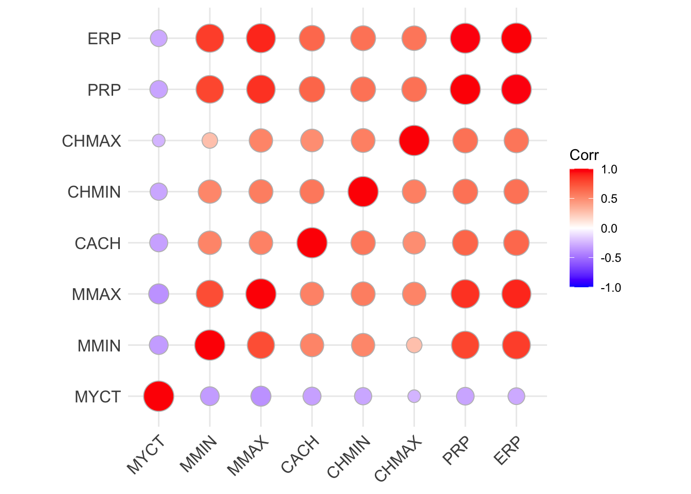

correlations = data.select_dtypes(include=np.number).corr(method='pearson')
with pd.option_context('display.max_columns', 40):
  print(correlations)

           MYCT      MMIN      MMAX      CACH     CHMIN     CHMAX       PRP       ERP
MYCT   1.000000 -0.335642 -0.378561 -0.321000 -0.301090 -0.250502 -0.307099 -0.288396
MMIN  -0.335642  1.000000  0.758157  0.534729  0.517189  0.266907  0.794931  0.819292
MMAX  -0.378561  0.758157  1.000000  0.537990  0.560513  0.527246  0.863004  0.901202
CACH  -0.321000  0.534729  0.537990  1.000000  0.582245  0.487846  0.662641  0.648620
CHMIN -0.301090  0.517189  0.560513  0.582245  1.000000  0.548281  0.608903  0.610580
CHMAX -0.250502  0.266907  0.527246  0.487846  0.548281  1.000000  0.605209  0.592156
PRP   -0.307099  0.794931  0.863004  0.662641  0.608903  0.605209  1.000000  0.966472
ERP   -0.288396  0.819292  0.901202  0.648620  0.610580  0.592156  0.966472  1.000000

names = data.select_dtypes(include=np.number).columns.values.tolist()
hmap=sns.heatmap(correlations, 
        xticklabels=correlations.columns,
        yticklabels=correlations.columns)
hmap.xaxis.tick_top()
plt.xticks(rotation=30)

(array([0.5, 1.5, 2.5, 3.5, 4.5, 5.5, 6.5, 7.5]), [Text(0.5, 1, 'MYCT'), Text(1.5, 1, 'MMIN'), Text(2.5, 1, 'MMAX'), Text(3.5, 1, 'CACH'), Text(4.5, 1, 'CHMIN'), Text(5.5, 1, 'CHMAX'), Text(6.5, 1, 'PRP'), Text(7.5, 1, 'ERP')])

plt.show()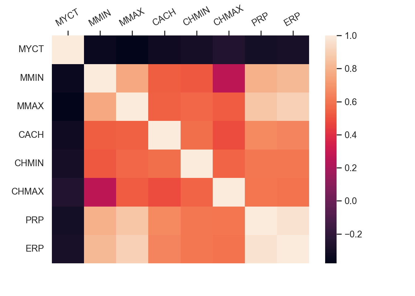

Observations

Some predictors (MYCT, MMIN, MMAX) have a large range of values as compared to others. Their standard deviation is high. As the predictors have different scales, data normalization may be needed, based on choice of model.
There is significant co-linearity between MMAX, MMIN and CACH.
The correlation plot indicates presence of collinearity between MMAX and MMIN. It also indicates strong positive correlation of the response PRP with MMAX and MMIN.
All the predictors have a significant right skew (especially MMIN, CHMIN and CHMAX).

Numeric Attributes

MYCT

R
Python

#MYCT,MMIN,MMAX,CACH,CHMIN,CHMAX,PRP,ERP
ggplot(data) + geom_density(aes(x=(MYCT)))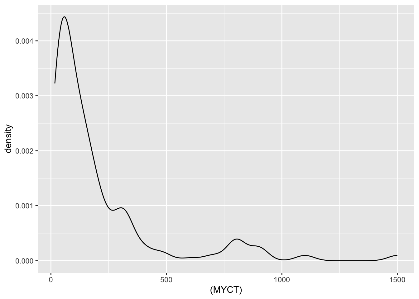

ggplot(data) + geom_boxplot(aes(y=factor(Vendor), x = MYCT))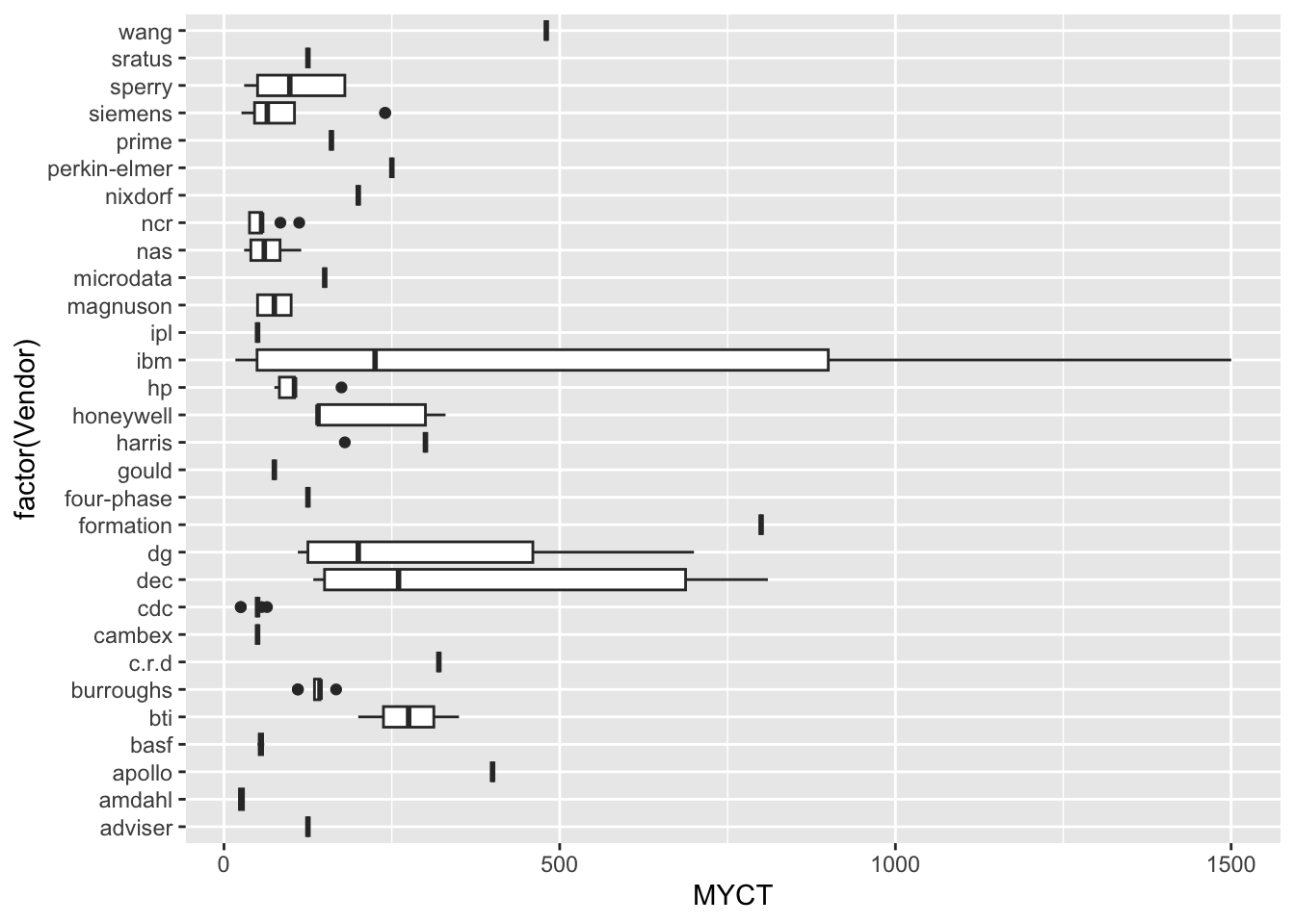

p = sns.displot(data, x="MYCT", kind="kde", height = 5, aspect = 1.5)
plt.show()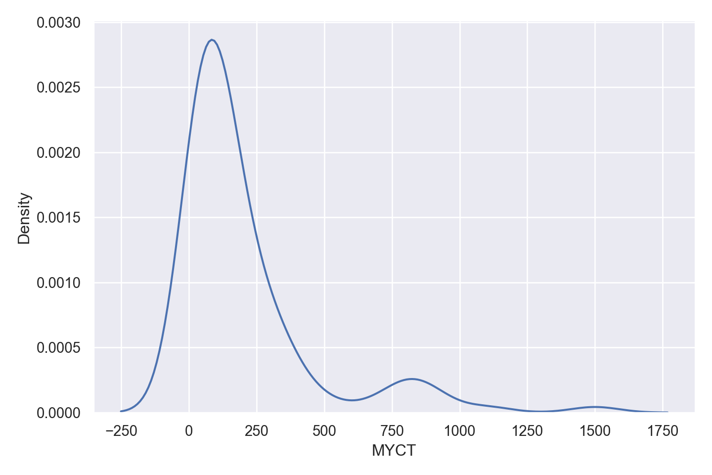

p = sns.catplot(data=data, y="Vendor", x="MYCT", kind="box", height = 5, aspect = 1.5)
plt.show()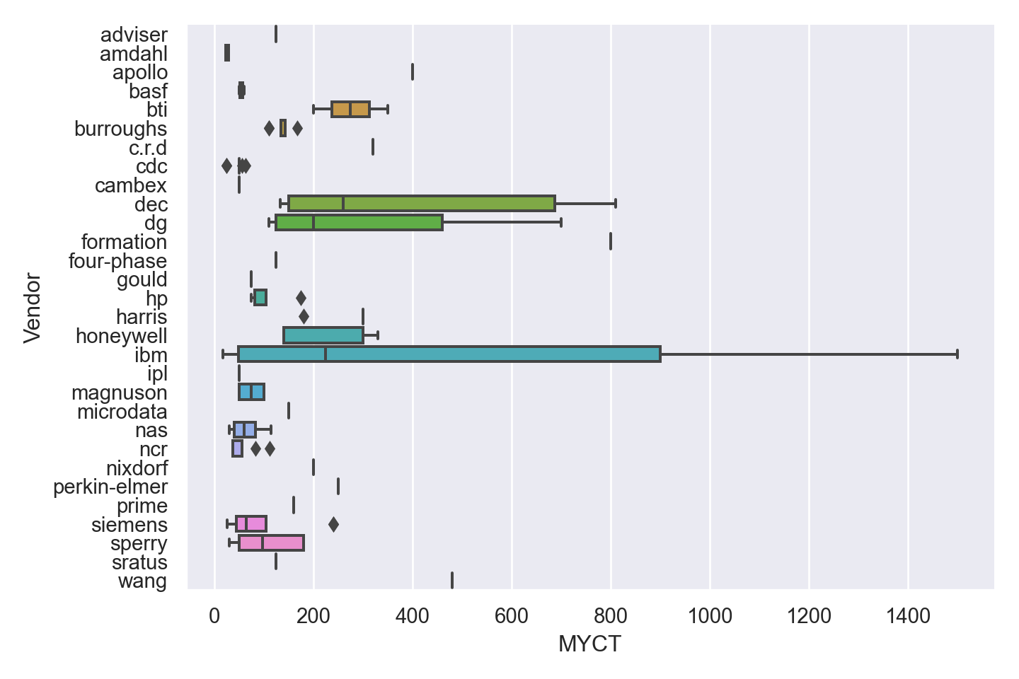

Observations

The density plot shows significant skew in the response values, as well as presence of outliers. However the data is valid and therefore cannot be removed for model fitting.
Some vendors (e.g. IBM) have models in a wider range of MYCT values, while others are more specialized.
IBM has an outlier model with very high MYCT.

MMIN

R
Python

ggplot(data) + geom_density(aes(x=(MMIN)))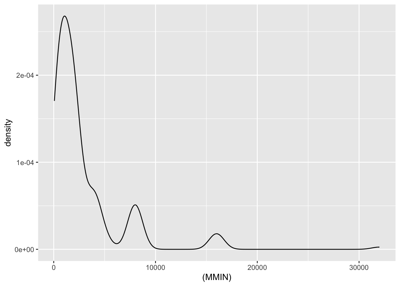

ggplot(data) + geom_boxplot(aes(y=factor(Vendor), x=MMIN))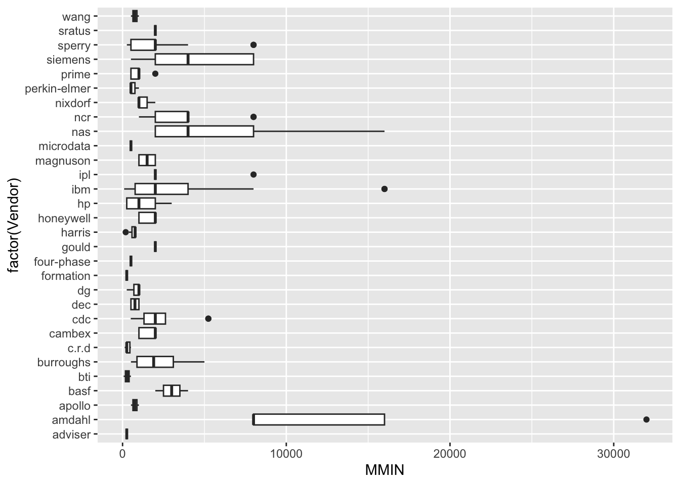

p=sns.displot(data, x="MMIN", kind="kde", height = 5, aspect = 1.5)
plt.show()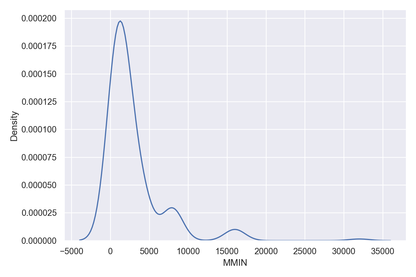

p=sns.catplot(data=data, x="MMIN", y="Vendor", kind="box", height = 5, aspect = 1.5)
plt.show()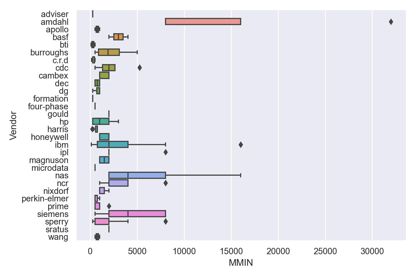

Observations

The density plot shows significant skew in the response values, as well as presence of outliers. However the data is valid and therefore cannot be removed for model fitting.
Some vendors (e.g. nas) have models in a wider range of MMIN values, while others are more specialized.
Amdahl has an outlier model with very high MMIN.

MMAX

R
Python

ggplot(data) + geom_density(aes(x=(MMAX)))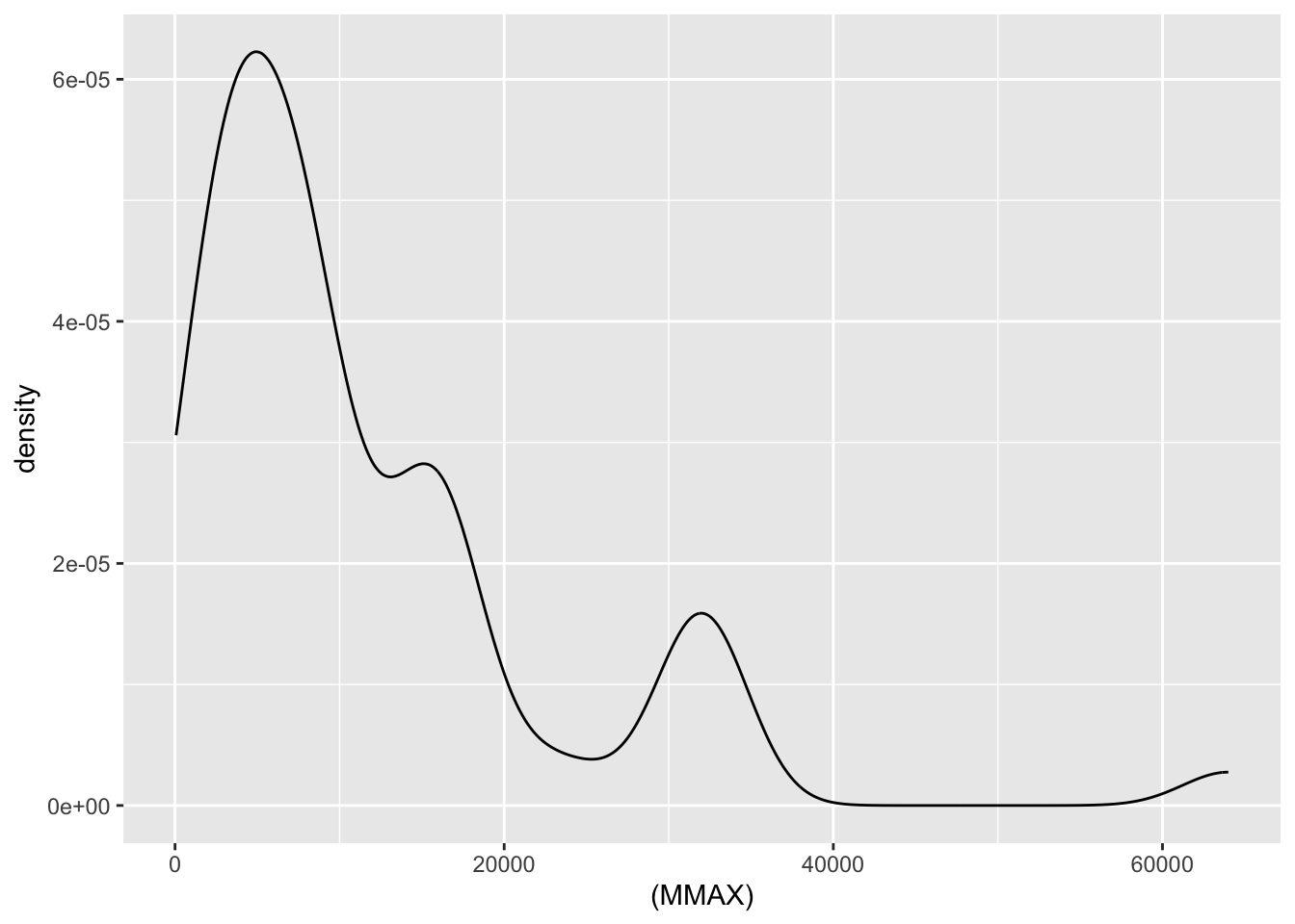

ggplot(data) + geom_boxplot(aes(y=factor(Vendor), x=MMAX))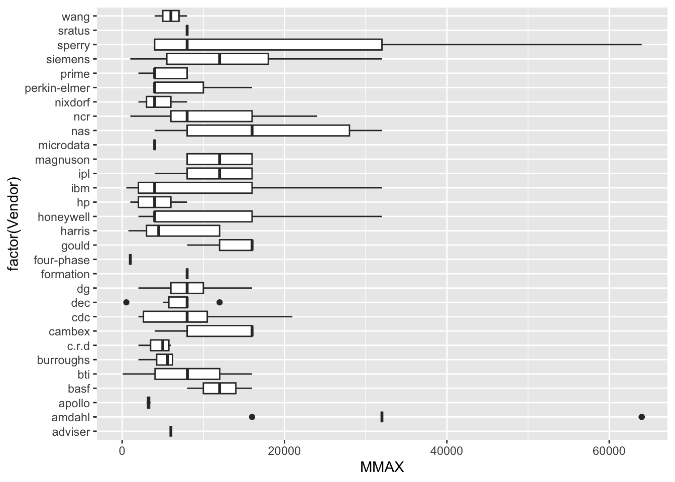

p=sns.displot(data, x="MMAX", kind="kde", height = 5, aspect = 1.5)
plt.show()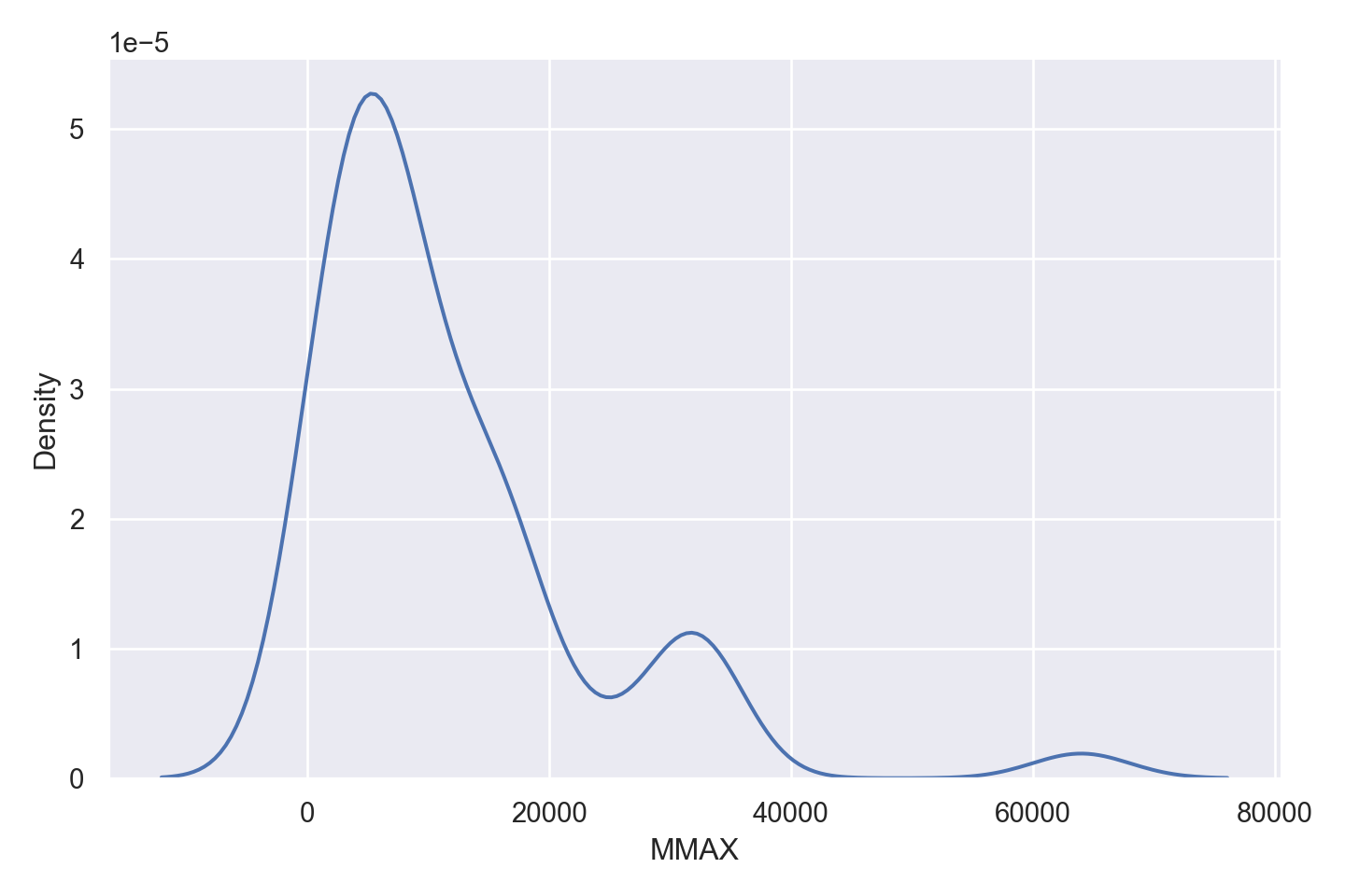

p=sns.catplot(data=data, x="MMAX", y="Vendor", kind="box", height = 5, aspect = 1.5)
plt.show()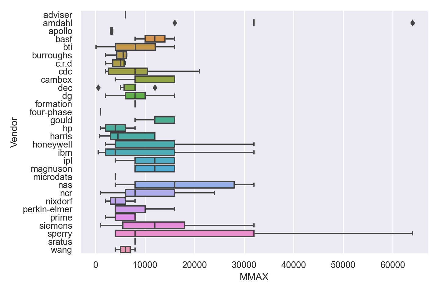

Observations

The density plot shows significant skew in the response values, as well as presence of outliers. However the data is valid and therefore cannot be removed for model fitting.
Some vendors (e.g. Sperry) have models in a wider range of MMAX values, while others are more specialized.
Sperry has an outlier model with very high MMAX.

CACH

R
Python

ggplot(data) + geom_density(aes(x=(CACH)))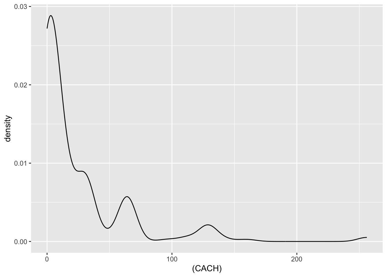

ggplot(data) + geom_boxplot(aes(y=factor(Vendor), x = CACH))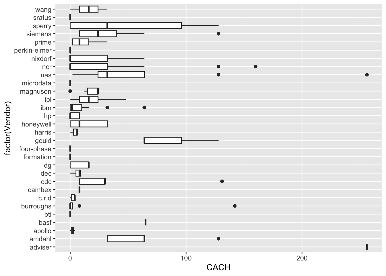

p=sns.displot(data, x="CACH", kind="kde", height = 5, aspect = 1.5)
plt.show()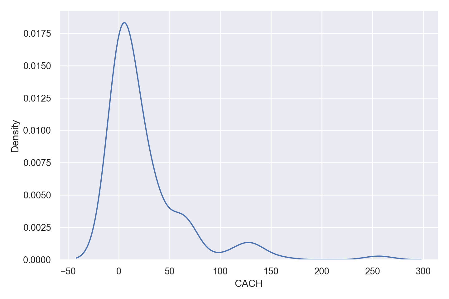

p=sns.catplot(data=data, x="CACH", y="Vendor", kind="box", height = 5, aspect = 1.5)
plt.show()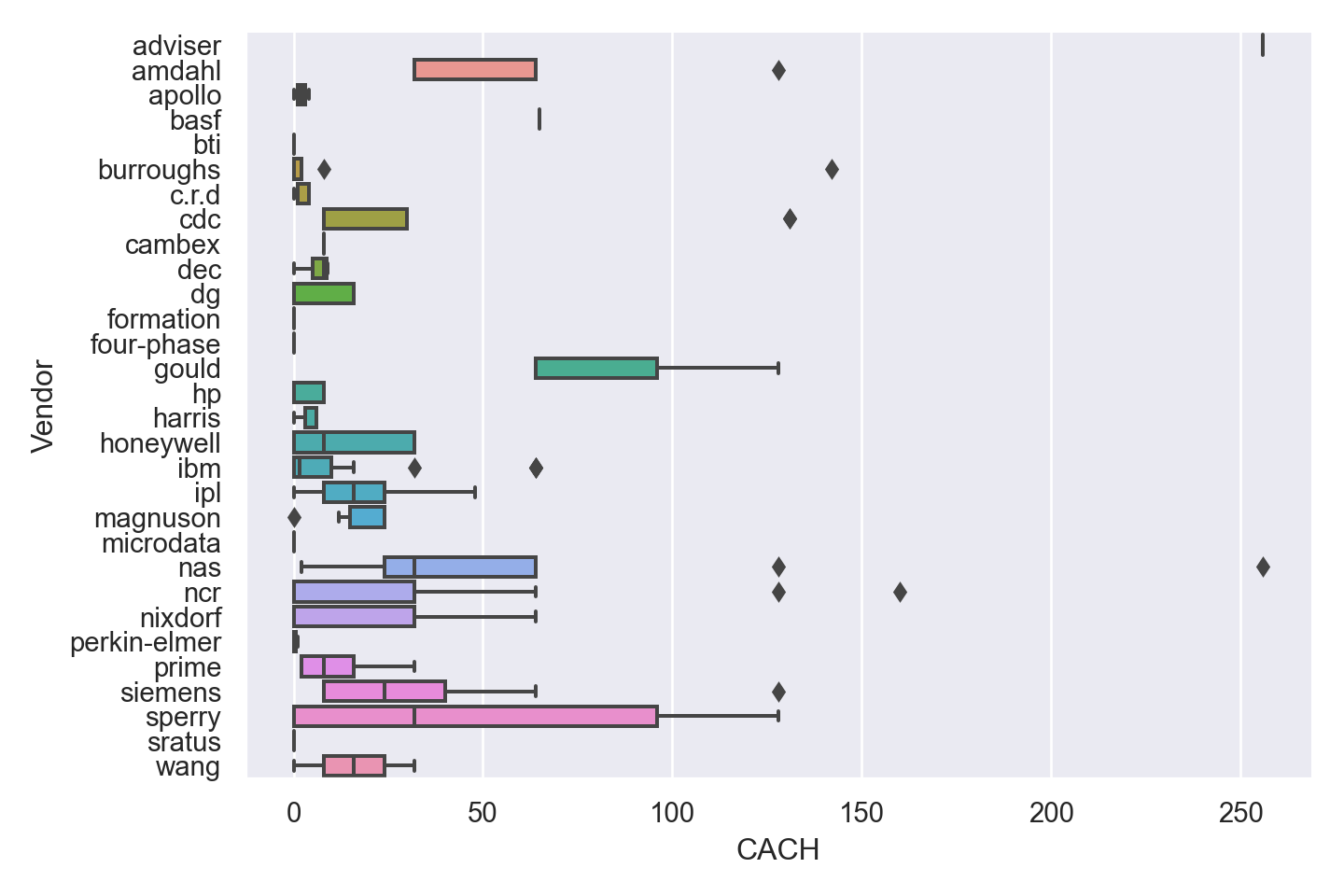

Observations

The density plot shows significant skew in the response values, as well as presence of outliers. However the data is valid and therefore cannot be removed for model fitting.
Some vendors (e.g. Sperry) have models in a wider range of CACH values, while others are more specialized.
NAS and Adviser have outlier models with very high MMAX.

CHMIN

R
Python

ggplot(data) + geom_density(aes(x=(CHMIN)))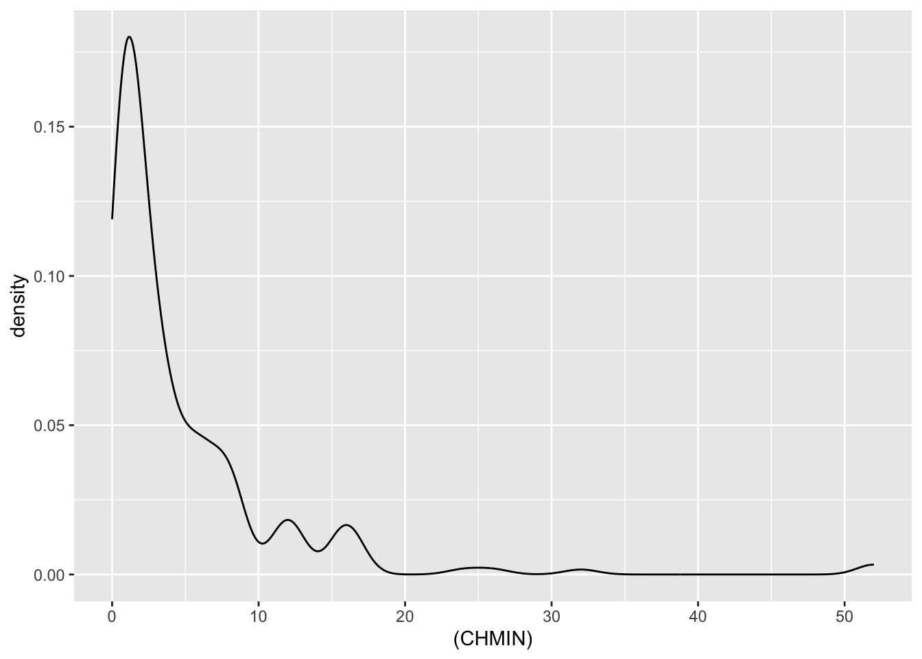

ggplot(data) + geom_boxplot(aes(y=factor(Vendor), x = CHMIN))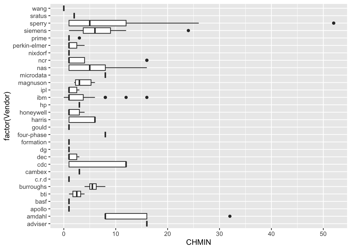

p=sns.displot(data, x="CHMIN", kind="kde", height = 5, aspect = 1.5)
plt.show()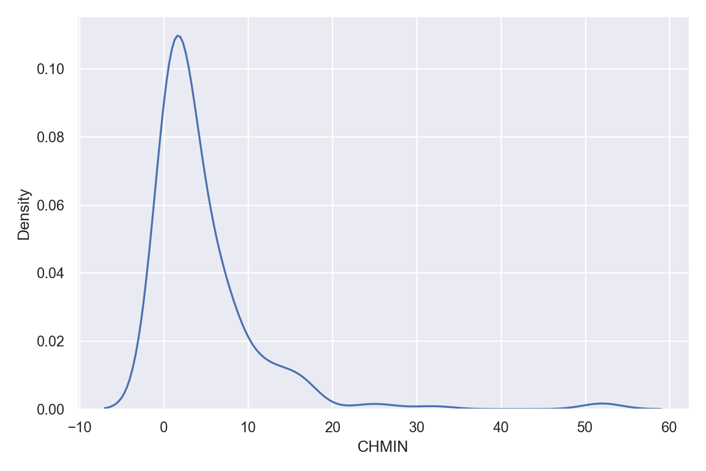

p=sns.catplot(data=data, x="CHMIN", y="Vendor", kind="box", height = 5, aspect = 1.5)
plt.show()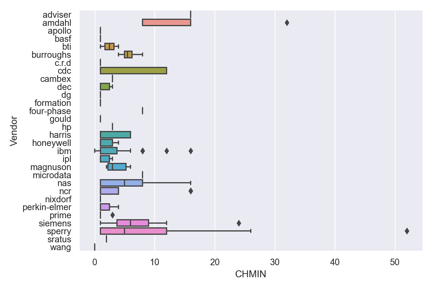

Observations

The density plot shows significant skew in the response values, as well as presence of outliers. However the data is valid and therefore cannot be removed for model fitting.
Some vendors (e.g. Sperry) have models in a wider range of CHMAX values, while others are more specialized.
Sperry and Amdahl have outlier models with very high CHMIN.

CHMAX

R
Python

#MYCT,MMIN,MMAX,CACH,CHMIN,CHMAX,PRP,ERP
ggplot(data) + geom_density(aes(x=(PRP)))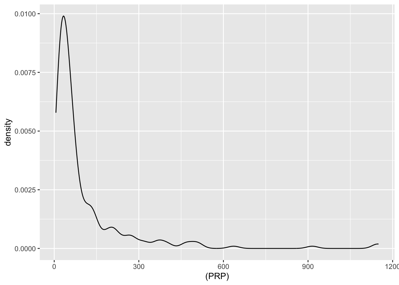

ggplot(data) + geom_boxplot(aes(y=factor(Vendor), x = PRP))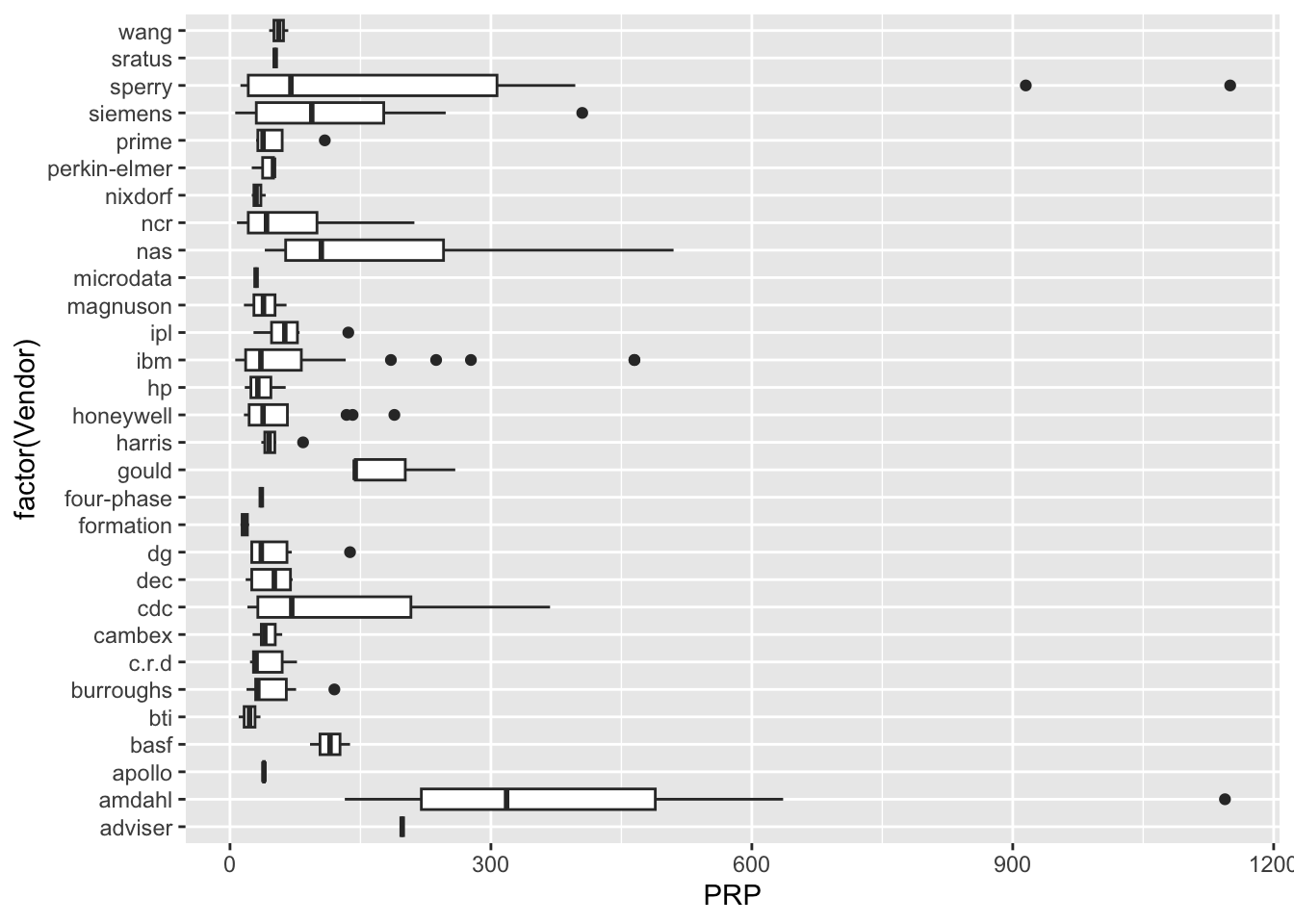

p=sns.displot(data, x="PRP", kind="kde", height = 5, aspect = 1.5)
plt.show()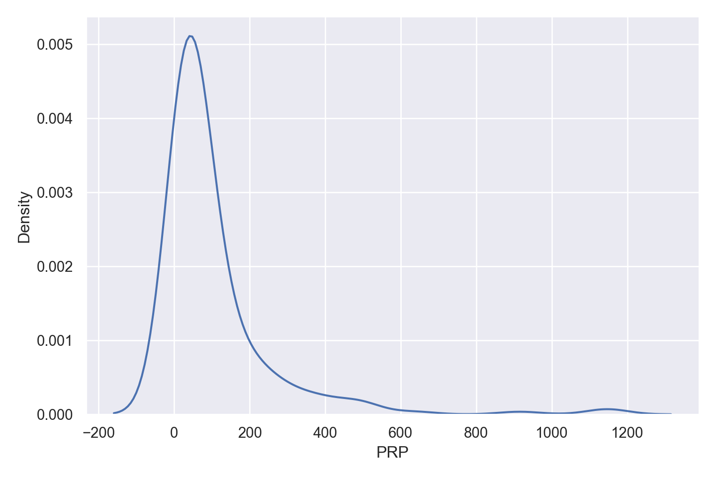

p=sns.catplot(data=data, x="PRP", y="Vendor", kind="box", height = 5, aspect = 1.5)
plt.show()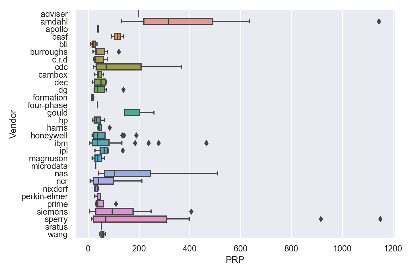

Observations

The density plot shows significant skew in the response values, as well as presence of outliers. However the data is valid and therefore cannot be removed for model fitting.
Some vendors (e.g. Amdahl) have models in a wider range of PRP values, while others are more narrow.
Sperry and Amdahl have outlier models with high PRP.

Training and Testing Split

R
Python

set.seed(83)

data_split = initial_split(data, prop = 3/4)

data_train = training(data_split)
data_test  = testing(data_split)

# Define the basic pre-processing recipe. This one does not have any predictor transformations or interactions.
machines_rec_1 = recipe(PRP ~ ., data = data_train) %>% 
                step_rm(ERP) %>%
                update_role(Model, new_role = "ID") %>%
                step_dummy(all_nominal_predictors())

# Define a recipe with transformations to reduce skewness
#machines_rec_1 = machines_rec_1 %>% step_BoxCox(all_numeric())
machines_rec_1 = machines_rec_1 %>% step_interact(terms = ~ CACH:CHMAX)

R
Python

# Model specifications

#Basic linear model
lm_basic_spec = linear_reg() %>% set_engine("lm")

#Generalized linear model with tuning
glm_spec  = linear_reg(penalty = tune(), mixture = tune()) %>% set_engine("glmnet")

linear_wfs = workflow_set(
                preproc = list(simple = machines_rec_1),
                models = list(basic = lm_basic_spec, glm = glm_spec)
            )

# Create 10 folds of the training data
data_folds = vfold_cv(data_train, strata = Vendor)

all_workflows = linear_wfs

grid_ctrl <-
   control_grid(
      save_pred = TRUE,
      parallel_over = "everything",
      save_workflow = TRUE
   )

grid_results <-
   linear_wfs %>%
   workflow_map(
      seed = 1503,
      resamples = data_folds,
      grid = 25,
      control = grid_ctrl
   )

grid_results %>% rank_results()

# A tibble: 52 × 9
   wflow_id     .config         .metric   mean std_err     n prepr…¹ model  rank
   <chr>        <chr>           <chr>    <dbl>   <dbl> <int> <chr>   <chr> <int>
 1 simple_basic Preprocessor1_… rmse    39.7    4.89      10 recipe  line…     1
 2 simple_basic Preprocessor1_… rsq      0.899  0.0254    10 recipe  line…     1
 3 simple_glm   Preprocessor1_… rmse    45.8    9.77      10 recipe  line…     2
 4 simple_glm   Preprocessor1_… rsq      0.886  0.0244    10 recipe  line…     2
 5 simple_glm   Preprocessor1_… rmse    45.8    9.77      10 recipe  line…     3
 6 simple_glm   Preprocessor1_… rsq      0.886  0.0244    10 recipe  line…     3
 7 simple_glm   Preprocessor1_… rmse    45.8    9.77      10 recipe  line…     4
 8 simple_glm   Preprocessor1_… rsq      0.886  0.0244    10 recipe  line…     4
 9 simple_glm   Preprocessor1_… rmse    45.8    9.77      10 recipe  line…     5
10 simple_glm   Preprocessor1_… rsq      0.886  0.0244    10 recipe  line…     5
# … with 42 more rows, and abbreviated variable name ¹preprocessor

best_results = grid_results %>% extract_workflow_set_result("simple_glm") %>% 
   select_best(metric = "rmse")

simple_glm_test_results <- 
   grid_results %>% 
   extract_workflow("simple_glm") %>% 
   finalize_workflow(best_results) %>% 
   last_fit(split = data_split)

final_fitted_model = simple_glm_test_results %>% extract_fit_parsnip()

simple_glm_test_results %>% collect_predictions() %>% arrange(.row)

# A tibble: 53 × 5
   id               .pred  .row   PRP .config             
   <chr>            <dbl> <int> <dbl> <chr>               
 1 train/test split 979.     10  1144 Preprocessor1_Model1
 2 train/test split -31.9    15    10 Preprocessor1_Model1
 3 train/test split 364.     20   120 Preprocessor1_Model1
 4 train/test split  43.1    21    30 Preprocessor1_Model1
 5 train/test split  32.0    25    23 Preprocessor1_Model1
 6 train/test split  23.2    26    69 Preprocessor1_Model1
 7 train/test split  35.1    29    77 Preprocessor1_Model1
 8 train/test split 124.     32   368 Preprocessor1_Model1
 9 train/test split 195.     35   106 Preprocessor1_Model1
10 train/test split  89.1    39    71 Preprocessor1_Model1
# … with 43 more rows

simple_linear_model_metrics = collect_metrics(simple_glm_test_results)
simple_linear_model_metrics

# A tibble: 2 × 4
  .metric .estimator .estimate .config             
  <chr>   <chr>          <dbl> <chr>               
1 rmse    standard      66.2   Preprocessor1_Model1
2 rsq     standard       0.924 Preprocessor1_Model1

# Find the metrics of existing estimated results
estimated_rmse=rmse(data_test, truth = PRP, estimate = ERP)
estimated_rsq=rsq(data_test, truth = PRP, estimate = ERP)

boxinvTransform <- function(y, lambda=-0.219) {
  if (lambda == 0L) { exp(y) }
  else { (y * lambda + 1)^(1/lambda) }
}

pred= as.tibble(simple_glm_test_results$.predictions[[1]]$.pred)
PRP = as.tibble(simple_glm_test_results$.predictions[[1]]$PRP)

#define plotting area
#op <- par(pty = "s", mfrow = c(1, 2))

#Q-Q plot for original model
#qqnorm(model$residuals)
#qqline(model$residuals)

#Q-Q plot for Box-Cox transformed model
#qqnorm(new_model$residuals)
#qqline(new_model$residuals)

#display both Q-Q plots
#par(op)


# Define the basic pre-processing recipe. This one does not have any predictor transformations or interactions.
machines_rec_2 = recipe(PRP ~ ., data = data_train) %>%
                step_novel(all_predictors(), -all_numeric()) %>%
                step_rm(ERP) %>%
                update_role(Model, new_role = "ID") %>%
                step_dummy(all_predictors(), -all_numeric()) 

decision_tree_spec = decision_tree(tree_depth = 5) %>% set_engine("rpart") %>% set_mode("regression")
boost_tree_spec = boost_tree(trees = 10) %>% set_engine("xgboost") %>% set_mode("regression")
rand_forest_spec = rand_forest(trees = 1000, mtry = tune()) %>% set_engine("randomForest") %>% set_mode("regression")

tree_wfs = workflow_set(
                preproc = list(simple = machines_rec_2),
                models = list(decision_tree = decision_tree_spec, boost_tree = boost_tree_spec, rand_forest = rand_forest_spec)
            )

grid_results <-
   tree_wfs %>%
   workflow_map(
      seed = 1503,
      resamples = data_folds,
      grid = 25,
      control = grid_ctrl
   )

grid_results %>% rank_results()

# A tibble: 52 × 9
   wflow_id           .config   .metric   mean std_err     n prepr…¹ model  rank
   <chr>              <chr>     <chr>    <dbl>   <dbl> <int> <chr>   <chr> <int>
 1 simple_rand_forest Preproce… rmse    44.3   12.5       10 recipe  rand…     1
 2 simple_rand_forest Preproce… rsq      0.863  0.0439    10 recipe  rand…     1
 3 simple_rand_forest Preproce… rmse    44.5   12.6       10 recipe  rand…     2
 4 simple_rand_forest Preproce… rsq      0.862  0.0438    10 recipe  rand…     2
 5 simple_rand_forest Preproce… rmse    44.5   12.5       10 recipe  rand…     3
 6 simple_rand_forest Preproce… rsq      0.862  0.0430    10 recipe  rand…     3
 7 simple_rand_forest Preproce… rmse    44.5   12.5       10 recipe  rand…     4
 8 simple_rand_forest Preproce… rsq      0.861  0.0437    10 recipe  rand…     4
 9 simple_rand_forest Preproce… rmse    44.6   12.7       10 recipe  rand…     5
10 simple_rand_forest Preproce… rsq      0.861  0.0434    10 recipe  rand…     5
# … with 42 more rows, and abbreviated variable name ¹preprocessor

best_results = grid_results %>% extract_workflow_set_result("simple_rand_forest") %>% 
   select_best(metric = "rmse")

simple_rf_test_results <- 
   grid_results %>% 
   extract_workflow("simple_rand_forest") %>% 
   finalize_workflow(best_results) %>% 
   last_fit(split = data_split)

final_fitted_rf_model = simple_rf_test_results %>% extract_fit_parsnip()

simple_rf_test_results %>% collect_predictions()

# A tibble: 53 × 5
   id               .pred  .row   PRP .config             
   <chr>            <dbl> <int> <dbl> <chr>               
 1 train/test split 631.     10  1144 Preprocessor1_Model1
 2 train/test split  16.7    15    10 Preprocessor1_Model1
 3 train/test split 175.     20   120 Preprocessor1_Model1
 4 train/test split  45.0    21    30 Preprocessor1_Model1
 5 train/test split  35.0    25    23 Preprocessor1_Model1
 6 train/test split  19.8    26    69 Preprocessor1_Model1
 7 train/test split  27.4    29    77 Preprocessor1_Model1
 8 train/test split 217.     32   368 Preprocessor1_Model1
 9 train/test split 180.     35   106 Preprocessor1_Model1
10 train/test split  46.9    39    71 Preprocessor1_Model1
# … with 43 more rows

simple_rf_model_metrics = collect_metrics(simple_rf_test_results)
simple_rf_model_metrics

# A tibble: 2 × 4
  .metric .estimator .estimate .config             
  <chr>   <chr>          <dbl> <chr>               
1 rmse    standard     104.    Preprocessor1_Model1
2 rsq     standard       0.906 Preprocessor1_Model1

machines_rec_norm = machines_rec_2

mlp_spec = mlp() %>% set_engine("nnet") %>% set_mode("regression")
svm_spec = svm_rbf() %>% set_engine("kernlab") %>% set_mode("regression")
rule_spec = rule_fit(trees = 1000) %>% set_engine("h2o") %>% set_mode("regression")


normalized_wfs = workflow_set(
                preproc = list(simple = machines_rec_norm),
                models = list(mlp = mlp_spec, svm = svm_spec)
            )

grid_results <-
   normalized_wfs %>%
   workflow_map(
      seed = 1503,
      resamples = data_folds,
      grid = 25,
      control = grid_ctrl
   )

grid_results %>% rank_results()

# A tibble: 4 × 9
  wflow_id   .config           .metric    mean std_err     n prepr…¹ model  rank
  <chr>      <chr>             <chr>     <dbl>   <dbl> <int> <chr>   <chr> <int>
1 simple_mlp Preprocessor1_Mo… rmse    120.    17.1       10 recipe  mlp       1
2 simple_mlp Preprocessor1_Mo… rsq       0.119  0.0442     2 recipe  mlp       1
3 simple_svm Preprocessor1_Mo… rmse    121.    21.1       10 recipe  svm_…     2
4 simple_svm Preprocessor1_Mo… rsq       0.333  0.0532    10 recipe  svm_…     2
# … with abbreviated variable name ¹preprocessor

best_results = grid_results %>% extract_workflow_set_result("simple_mlp") %>% 
   select_best(metric = "rmse")

simple_mlp_test_results <- 
   grid_results %>% 
   extract_workflow("simple_mlp") %>% 
   finalize_workflow(best_results) %>% 
   last_fit(split = data_split)

final_fitted_mlp_model = simple_mlp_test_results %>% extract_fit_parsnip()

simple_mlp_test_results %>% collect_predictions()

# A tibble: 53 × 5
   id               .pred  .row   PRP .config             
   <chr>            <dbl> <int> <dbl> <chr>               
 1 train/test split  97.8    10  1144 Preprocessor1_Model1
 2 train/test split  15.0    15    10 Preprocessor1_Model1
 3 train/test split  97.8    20   120 Preprocessor1_Model1
 4 train/test split  97.8    21    30 Preprocessor1_Model1
 5 train/test split  97.8    25    23 Preprocessor1_Model1
 6 train/test split  97.8    26    69 Preprocessor1_Model1
 7 train/test split  97.8    29    77 Preprocessor1_Model1
 8 train/test split  97.8    32   368 Preprocessor1_Model1
 9 train/test split  97.8    35   106 Preprocessor1_Model1
10 train/test split  97.8    39    71 Preprocessor1_Model1
# … with 43 more rows

simple_mlp_model_metrics = collect_metrics(simple_rf_test_results)
simple_mlp_model_metrics

# A tibble: 2 × 4
  .metric .estimator .estimate .config             
  <chr>   <chr>          <dbl> <chr>               
1 rmse    standard     104.    Preprocessor1_Model1
2 rsq     standard       0.906 Preprocessor1_Model1

The GLM model without any interaction terms gives the best results with RMSE = 66.22 and R-squared = 0.9235.